On Balance Volume [BrightSideTrading]
# On Balance Volume - Complete User Guide
## Overview
This enhanced OBV indicator provides clean, actionable volume analysis with intelligent signal filtering. It combines On-Balance Volume (OBV) with a smoothed signal line to identify shifts in buying and selling pressure without chart clutter.
**Key Features:**
- Real-time OBV and signal line visualization
- Smart crossover detection with confirmation filtering
- Z-Score momentum analysis
- Customizable signal alerts with V-shaped markers
- Window-normalized option for detrended analysis
---
## What is On-Balance Volume (OBV)?
OBV is a volume-based momentum indicator that accumulates volume on up days and subtracts volume on down days. It answers a fundamental question: **Is volume flowing in (buying) or out (selling)?**
**Formula:**
- If Close > Previous Close: OBV = Previous OBV + Volume
- If Close < Previous Close: OBV = Previous OBV - Volume
- If Close = Previous Close: OBV = Previous OBV (unchanged)
**What it tells you:**
- **Rising OBV** = Accumulation (smart money buying)
- **Falling OBV** = Distribution (smart money selling)
- **OBV above zero line** = Net positive buying pressure
- **OBV below zero line** = Net negative selling pressure
---
## Interface & Settings
### **MAIN VISUALIZATION**
**OBV Line (Green/Red Ribbon)**
- Green when OBV is above the signal line (bullish trend)
- Red when OBV is below the signal line (bearish trend)
- Toggles between window-normalized (detrended) and raw values
**Signal Line (Orange)**
- Smoothed average of OBV
- Crossovers with OBV generate buy/sell signals
- Default: 21-period SMA
**V-Shaped Markers**
- Green upward V = Bullish crossover (buy signal)
- Red downward V = Bearish crossover (sell signal)
- Appears at the OBV value when signal is triggered
**Zero Line (Yellow)**
- Center equilibrium point for volume balance
- Acts as support/resistance for OBV
- Separates buying pressure (above) from selling pressure (below)
---
### **SOURCE GROUP**
**Source**
- **Default:** Close
- **Options:** Open, High, Low, or any custom value
- Controls which price value triggers OBV direction changes
- Most traders use Close for standard OBV calculation
---
### **SIGNAL SMOOTHING GROUP**
**Show Signal?**
- **Default:** ON
- Toggle visibility of the signal line
- Disable if you prefer to see raw OBV only
**Smoothing Type**
- **SMA (Simple Moving Average)** - Default, standard smoothing
- **EMA (Exponential Moving Average)** - Faster response, weights recent bars more heavily
- **Choose SMA** for consistent, traditional OBV signals
- **Choose EMA** for faster trend identification (more whipsaws possible)
**Smoothing Length**
- **Default:** 21 bars
- **Range:** 1-200 bars
- **Lower values** (5-14): Faster signals, more noise
- **Higher values** (30-50): Slower signals, fewer false alarms
- **Recommendation:** Use 21-25 for most timeframes
---
### **SIGNAL FILTERING GROUP**
This is your primary control for signal quality and frequency.
**Show Signal Markers?**
- **Default:** ON
- Toggle the V-shaped buy/sell markers on/off
- Disable if markers distract from your analysis
**Signal Filter Type**
- **None** - Shows every single crossover (noisy, best for skilled traders)
- **Confirmation Bars** - Waits N bars before confirming signal (recommended)
- **Strength-Based** - Only signals during strong momentum (filters weakest moves)
#### **CONFIRMATION BARS MODE** (Recommended)
Best for reducing false signals while staying responsive to real moves.
**Confirmation Bars**
- **Default:** 2 bars
- **Range:** 1-10 bars
- Waits for the signal to hold for N consecutive bars after crossover
- **Setting 1:** Every crossover (same as "None")
- **Setting 2:** Wait 1 bar confirmation (good balance)
- **Setting 3:** Wait 2 bars confirmation (filters 50% of noise)
- **Setting 4+:** Very selective, misses quick reversals
**How it works:**
1. OBV crosses signal line → Confirmation counter starts
2. If OBV stays on correct side for 2 bars → V-marker appears
3. If OBV crosses back → Counter resets, no signal
#### **STRENGTH-BASED MODE**
Only signals when momentum is statistically significant.
**Min Z-Score Strength**
- **Default:** 0.3
- **Range:** 0.0-3.0
- Requires OBV deviation from its mean to reach this threshold
- **Setting 0.1-0.3:** More signals, lower quality
- **Setting 0.5-0.8:** Moderate signals, good quality
- **Setting 1.0+:** Only the strongest momentum shifts
**How it works:**
- Calculates how far OBV is from its 50-bar average (Z-score)
- Only shows signals when this distance is meaningful
- Automatically avoids weak, choppy market conditions
---
### **VISUALS & COLORS GROUP**
**Highlight Crossovers?**
- **Default:** ON
- Master toggle for all signal markers
- Turn OFF to see only the OBV/signal lines
**Apply Ribbon Filling?**
- **Default:** ON
- Colors the space between OBV and signal line
- Green fill = OBV above signal (bullish)
- Red fill = OBV below signal (bearish)
- Provides clear visual trend confirmation
- Turn OFF for minimal chart clutter
---
### **STATS & ZONES GROUP**
**Use Window-Normalized OBV (visual only)?**
- **Default:** ON
- Removes long-term trend from OBV for clearer short-term signals
- Detrends the indicator to highlight recent momentum changes
- **ON:** Better for swing trading and identifying reversals
- **OFF:** Better for trend-following strategies
- Note: Z-Score always uses raw OBV for statistical accuracy
**OBV Normalize Window**
- **Default:** 200 bars
- Lookback period for detrending calculation
- Larger values = more aggressive detrending
- Adjust if you want OBV to oscillate more/less around zero
**Show Z-Score (OBV)?**
- **Default:** ON
- Displays statistical momentum indicator below main chart
- Ranges from -3 to +3 (most data within -2 to +2)
- High Z-Score = Strong buying momentum
- Low Z-Score = Strong selling momentum
**Z-Score Lookback**
- **Default:** 50 bars
- Period for calculating Z-Score mean and standard deviation
- Larger = smoother Z-Score, slower response
- Smaller = noisier Z-Score, faster response
**Show ROC (OBV Momentum)?**
- **Default:** OFF
- Rate of Change indicator for OBV velocity
- Useful for identifying momentum turning points
- Enable if you want to see speed of volume changes
**ROC Lookback**
- **Default:** 14 bars
- Period for ROC calculation
**Show Z-Score StdDev Zones?**
- **Default:** ON
- Shaded regions around zero line showing statistical boundaries
- Inner Zone (±1 Z) = Normal variation
- Outer Zone (±2 Z) = Extreme moves, potential reversals
- Helps identify overbought/oversold volume conditions
**Inner Zone (±Z)**
- **Default:** 1.0
- First boundary for standard deviation zones
- Most normal trading occurs within ±1
**Outer Zone (±Z)**
- **Default:** 2.0
- Second boundary for extreme conditions
- Crossing these zones indicates significant momentum shift
---
## Trading Strategy Examples
### **Strategy 1: Signal Line Crossovers (Beginner)**
**Setup:**
- Signal Filter Type: **Confirmation Bars**
- Confirmation Bars: **2-3**
- Show Signal Markers: **ON**
**Rules:**
1. **BUY signal** (green V): When OBV crosses above signal line and holds for 2-3 bars
- Confirms buying pressure is building
- Look for price to follow within 1-3 bars
2. **SELL signal** (red V): When OBV crosses below signal line and holds for 2-3 bars
- Confirms selling pressure is increasing
- Expect price decline
3. **Exit:** Take profits at next signal or use price support/resistance
**Best For:** Swing trading, intraday reversals, timeframes 5m-1h
---
### **Strategy 2: Zero Line Bounce (Intermediate)**
**Setup:**
- Signal Filter Type: **Strength-Based**
- Min Z-Score Strength: **0.5**
- Show Z-Score StdDev Zones: **ON**
**Rules:**
1. **Watch OBV approach zero line** during established trends
- OBV bouncing repeatedly off zero = trend is healthy
- OBV breaking through zero = trend reversal imminent
2. **Enter on bounce:** Buy when OBV bounces from zero line in uptrend
3. **Exit on break:** Close position when OBV breaks below zero line
4. **Confirm with Z-Score:** Only take trades when Z-Score shows momentum (|Z| > 0.5)
**Best For:** Trend traders, identifying trend strength, medium timeframes 15m-4h
---
### **Strategy 3: Momentum Extremes (Advanced)**
**Setup:**
- Signal Filter Type: **None**
- Show Z-Score StdDev Zones: **ON**
- Outer Zone: **2.0**
**Rules:**
1. **Identify extremes:** When Z-Score breaks outer zone (±2.0)
- Indicator is in extreme territory
- Likely overextended
2. **Fade extremes:** Take opposite position when Z-Score hits extreme
- High Z (>2.0) = OBV overbought, expect pullback
- Low Z (<-2.0) = OBV oversold, expect bounce
3. **Confirm:** Wait for crossover signal to enter
4. **Target:** Outer zone of opposite side or zero line
**Best For:** Range trading, mean reversion, experienced traders only
---
## Reading the Indicator in Different Markets
### **Strong Uptrend**
- OBV consistently above signal line (green)
- OBV well above zero line, rising higher lows
- Z-Score positive, trending upward
- **Action:** Buy dips to signal line, sell at resistance
### **Strong Downtrend**
- OBV consistently below signal line (red)
- OBV well below zero line, making lower highs
- Z-Score negative, trending downward
- **Action:** Sell rallies to signal line, cover at support
### **Consolidation/Choppy Market**
- OBV whipsaws around signal line frequently
- Crossovers occur every few bars
- Z-Score oscillating between -1 and +1
- **Action:** Increase confirmation bars to 3-4, or switch to strength-based filter
### **Accumulation (Bottom Formation)**
- OBV rising while price is flat or falling
- Volume flowing in despite downtrend (bullish divergence)
- Z-Score climbing while price lows hold
- **Action:** Expect breakout up; prepare buy near support
### **Distribution (Top Formation)**
- OBV falling while price is flat or rising
- Volume flowing out despite uptrend (bearish divergence)
- Z-Score falling while price continues higher
- **Action:** Expect breakdown down; prepare short near resistance
---
## Parameter Tuning Guide
### **Aggressive Settings (More Signals)**
- Smoothing Length: 14
- Signal Filter: None or Confirmation Bars: 1
- Min Z-Score: 0.1
- Best for: Day trading, high volatility stocks
- Risk: More false signals
### **Balanced Settings (Recommended)**
- Smoothing Length: 21
- Signal Filter: Confirmation Bars: 2
- Min Z-Score: 0.3
- Best for: Swing trading, most market conditions
- Risk/Reward: Moderate
### **Conservative Settings (Fewer Signals)**
- Smoothing Length: 30-40
- Signal Filter: Confirmation Bars: 3-4 or Strength-Based: 0.7+
- Min Z-Score: 0.8
- Best for: Position trading, high-conviction trades only
- Risk: May miss some moves
---
## Common Questions & Troubleshooting
**Q: Why are there more sell signals than buy signals?**
A: This reflects the actual market action. Markets often decline faster than they rise (fear > greed). Confirm signals with price action and support/resistance.
**Q: The indicator keeps whipsawing, should I hide it?**
A: Increase Confirmation Bars to 3-4 or switch to Strength-Based filter. Market conditions matter—choppy markets require stricter filters.
**Q: What's the difference between normalized and raw OBV?**
A: Normalized (detrended) shows shorter-term momentum by removing long-term trends. Raw OBV shows absolute accumulation/distribution over the full period. Use normalized for swing signals, raw for trend confirmation.
**Q: My signals come too late. How do I get faster entry?**
A: Reduce Smoothing Length (try 14 instead of 21), use EMA instead of SMA, or set Confirmation Bars to 1. Trade-off: More false signals.
**Q: Can I use this for day trading?**
A: Yes, on 1m-5m charts with aggressive settings. Use Confirmation Bars: 1 and focus on Z-Score > 0.5 entries only.
**Q: Should I trade every signal?**
A: No. Filter signals using: price near support/resistance, multiple indicators confirming, and Z-Score showing momentum. Best signals occur at key levels.
---
## Best Practices
1. **Always confirm with price action:** OBV signals work best when price is near support, resistance, or moving average. Don't trade signals in a vacuum.
2. **Use volume context:** Check if volume is increasing or decreasing on the signal. Strong signals have volume confirmation (increasing volume on OBV spikes).
3. **Adjust settings per timeframe:**
- 1m-5m: Smoothing 12, Confirmation 1, Z-Score 0.2
- 15m-1h: Smoothing 20, Confirmation 2, Z-Score 0.3
- 4h-1d: Smoothing 25, Confirmation 3, Z-Score 0.5
4. **Watch the zero line:** It's your friend. OBV behavior at the zero line reveals trend strength. Bounces = healthy trend. Breaks = reversal.
5. **Risk management:** No indicator is perfect. Use proper position sizing and stop losses. OBV should confirm your thesis, not be the only reason to trade.
6. **Combine with other indicators:**
- Price moving averages for trend confirmation
- RSI or Stochastic for overbought/oversold levels
- Support/resistance for entry/exit zones
- MACD for momentum divergences
---
## Disclaimer
This indicator is for educational and informational purposes only. It is not financial advice. Past performance does not guarantee future results. Always conduct your own research and consult with a financial advisor before making trading decisions. Trading carries risk, including potential loss of principal.
---
## Version History
**Version 1.0** - Initial release with enhanced signal filtering, Z-Score analysis, and customizable parameters.
Cerca negli script per "Exponential Moving Average"

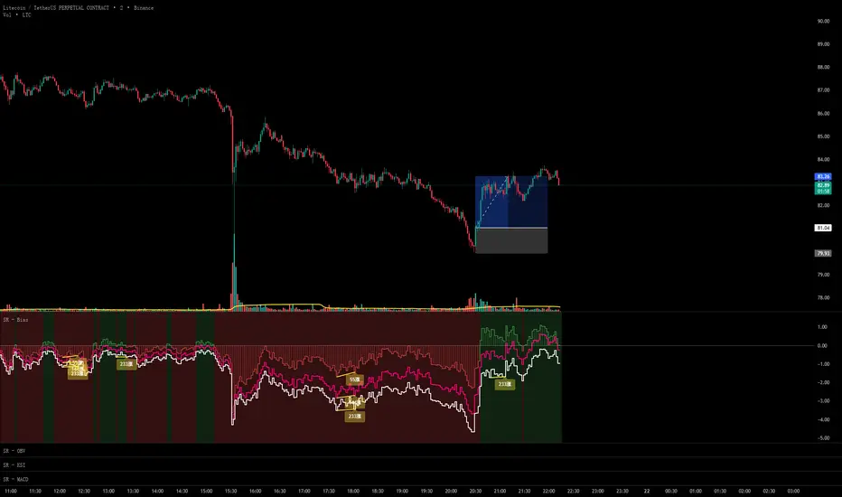
Scout Regiment - Bias# Scout Regiment - Bias Indicator
## English Documentation
### Overview
Scout Regiment - Bias is a technical indicator that measures the deviation (bias) between the current price and exponential moving averages (EMAs). It helps traders identify overbought/oversold conditions, trend strength, and potential reversal points through divergence detection.
### What is Bias?
Bias measures how far the price has moved away from a moving average, expressed as a percentage:
- **Positive Bias**: Price is above the EMA (potential overbought)
- **Negative Bias**: Price is below the EMA (potential oversold)
- **Formula**: Bias = (Price - EMA) / EMA × 100
### Key Features
#### 1. **Triple EMA Bias Lines**
The indicator calculates bias from three different EMAs:
- **EMA 55 Bias** (Default: Green/Red, 1px line)
- Short-term bias measurement
- Quick response to price changes
- Best for intraday and swing trading
- **EMA 144 Bias** (Pink, 2px line)
- Medium-term bias measurement
- Balanced response to price movements
- Ideal for swing trading
- **EMA 233 Bias** (White, 2px line)
- Long-term bias measurement
- Slower response, more stable
- Best for position trading
**Color Coding:**
- Green: Price above EMA (bullish)
- Red: Price below EMA (bearish)
#### 2. **Visual Components**
**Histogram Display**
- Shows EMA 55 bias as a histogram for easy visualization
- Green bars: Price above EMA 55
- Red bars: Price below EMA 55
- Can be toggled on/off
**Background Color**
- Light green background: Bullish bias (price above EMA 55)
- Light red background: Bearish bias (price below EMA 55)
- Optional display for cleaner charts
**Zero Line**
- White horizontal line at 0%
- Reference point for positive/negative bias
- Crossovers indicate trend changes
**Crossover Labels**
- "突破" (Breakout): When bias crosses above zero
- "跌破" (Breakdown): When bias crosses below zero
- Can be enabled/disabled for clarity
#### 3. **Divergence Detection**
The indicator automatically detects regular divergences for all three bias lines:
**Bullish Divergence (Yellow Labels)**
- Price makes lower lows
- Bias makes higher lows
- Suggests potential upward reversal
- Labels: "55涨", "144涨", "233涨"
**Bearish Divergence (Blue Labels)**
- Price makes higher highs
- Bias makes lower highs
- Suggests potential downward reversal
- Labels: "55跌", "144跌", "233跌"
**Divergence Parameters** (Customizable for each EMA):
- Left Lookback: Bars to the left of pivot (default: 5)
- Right Lookback: Bars to the right of pivot (default: 1)
- Max Lookback Range: Maximum distance between pivots (default: 60)
- Min Lookback Range: Minimum distance between pivots (default: 5)
### Configuration Settings
#### Bias Settings
- **EMA Periods**: Customize lengths for EMA 55, 144, and 233
- **Price Source**: Choose calculation source (default: close)
- **Enable/Disable**: Toggle each bias line independently
#### Display Settings
- **Show Histogram**: Toggle histogram display
- **Show Background Color**: Toggle background coloring
- **Show Crossover Labels**: Toggle breakout/breakdown labels
#### Divergence Settings (Per EMA)
- Individual controls for EMA 55, 144, and 233 divergences
- Customizable lookback parameters for precision tuning
- Adjustable range settings for different market conditions
### How to Use
#### For Trend Trading
1. **Identify Trend Direction**
- Price above zero = Uptrend
- Price below zero = Downtrend
2. **Confirm with Multiple Timeframes**
- EMA 55: Short-term trend
- EMA 144: Medium-term trend
- EMA 233: Long-term trend
3. **Trade in Direction of Bias**
- All three lines positive = Strong uptrend
- All three lines negative = Strong downtrend
#### For Mean Reversion Trading
1. **Identify Extremes**
- High positive bias (>5-10%) = Overbought
- High negative bias (<-5 to -10%) = Oversold
2. **Wait for Confirmation**
- Look for bias to turn back toward zero
- Watch for crossover labels
3. **Enter on Reversal**
- Enter long when extreme negative bias starts rising
- Enter short when extreme positive bias starts falling
#### For Divergence Trading
1. **Spot Divergence Labels**
- Yellow labels = Bullish divergence (potential buy)
- Blue labels = Bearish divergence (potential sell)
2. **Confirm with Price Action**
- Wait for price to confirm with structure break
- Look for support/resistance reactions
3. **Use Multiple EMAs**
- EMA 55 divergence: Quick reversals
- EMA 144 divergence: Reliable signals
- EMA 233 divergence: Major trend changes
#### For Multi-Timeframe Analysis
1. **Check Long-term Bias** (EMA 233)
- Determines overall market direction
2. **Find Medium-term Entry** (EMA 144)
- Look for pullbacks in long-term trend
3. **Time Short-term Entry** (EMA 55)
- Enter when short-term aligns with longer timeframes
### Trading Strategies
#### Strategy 1: Triple Confirmation
- Wait for all three bias lines to be positive (or negative)
- Enter in direction of unanimous bias
- Exit when any line crosses zero
- Best for: Strong trending markets
#### Strategy 2: Divergence Trading
- Enable all divergence detection
- Take trades only when divergence appears
- Confirm with price structure
- Best for: Range-bound and reversal setups
#### Strategy 3: Zero Line Crossover
- Enable crossover labels
- Enter long on "突破" labels
- Enter short on "跌破" labels
- Use stop loss at recent swing points
- Best for: Trend following
#### Strategy 4: Extreme Reversion
- Wait for bias to reach extremes (>10% or <-10%)
- Enter counter-trend when bias reverses
- Exit at zero line
- Best for: Ranging markets
### Best Practices
1. **Combine with Price Action**
- Don't trade bias alone
- Confirm with support/resistance
- Look for candlestick patterns
2. **Use Multiple Timeframes**
- Check higher timeframe bias
- Trade in direction of larger trend
- Use lower timeframe for entry timing
3. **Manage Risk**
- Set stop losses beyond recent swings
- Don't fight extreme bias in strong trends
- Reduce position size at extremes
4. **Customize for Your Market**
- Volatile assets: Use wider ranges
- Stable assets: Use tighter ranges
- Adjust EMA periods for your timeframe
5. **Watch for False Signals**
- Multiple small divergences = Less reliable
- Divergences at extremes = More reliable
- Confirm with other indicators
### Indicator Combinations
**With Volume:**
- High bias + Low volume = Weak move
- High bias + High volume = Strong move
**With Moving Averages:**
- Check if price is above/below key EMAs
- Bias confirms EMA trend strength
**With RSI/MACD:**
- Multiple indicator divergence = Stronger signal
- Use bias for overbought/oversold confirmation
### Performance Tips
- Disable unused features for faster loading
- Use histogram for quick visual reference
- Enable background color for trend clarity
- Use divergence detection selectively
### Common Patterns
1. **Bias Expansion**: Bias increasing = Strong trend
2. **Bias Contraction**: Bias decreasing = Trend weakening
3. **Zero Line Bounce**: Price respects EMA as support/resistance
4. **Extreme Bias**: Over-extension, watch for reversal
5. **Divergence Cluster**: Multiple EMAs diverging = High probability reversal
### Alert Conditions
You can set alerts for:
- Bias crossing above/below zero
- Extreme bias levels
- Divergence detection
- All three bias lines aligned
---
## 中文说明文档
### 概述
Scout Regiment - Bias 是一个技术指标,用于测量当前价格与指数移动平均线(EMA)之间的偏离程度(乖离率)。它帮助交易者识别超买超卖状况、趋势强度,以及通过背离检测发现潜在的反转点。
### 什么是乖离率?
乖离率衡量价格偏离移动平均线的程度,以百分比表示:
- **正乖离**:价格高于EMA(可能超买)
- **负乖离**:价格低于EMA(可能超卖)
- **计算公式**:乖离率 = (价格 - EMA) / EMA × 100
### 核心功能
#### 1. **三重EMA乖离率线**
指标计算三条不同EMA的乖离率:
- **EMA 55 乖离率**(默认:绿色/红色,1像素线)
- 短期乖离测量
- 对价格变化反应快速
- 适合日内和波段交易
- **EMA 144 乖离率**(粉色,2像素线)
- 中期乖离测量
- 对价格波动反应平衡
- 最适合波段交易
- **EMA 233 乖离率**(白色,2像素线)
- 长期乖离测量
- 反应较慢,更稳定
- 适合仓位交易
**颜色编码:**
- 绿色:价格高于EMA(看涨)
- 红色:价格低于EMA(看跌)
#### 2. **视觉组件**
**柱状图显示**
- 以柱状图形式显示EMA 55乖离率,便于可视化
- 绿色柱:价格高于EMA 55
- 红色柱:价格低于EMA 55
- 可开关显示
**背景颜色**
- 浅绿色背景:看涨乖离(价格高于EMA 55)
- 浅红色背景:看跌乖离(价格低于EMA 55)
- 可选显示,图表更清爽
**零轴**
- 零点位置的白色横线
- 正负乖离的参考点
- 穿越表示趋势变化
**穿越标签**
- "突破":乖离率向上穿越零轴
- "跌破":乖离率向下穿越零轴
- 可启用/禁用以保持清晰
#### 3. **背离检测**
指标自动检测所有三条乖离率线的常规背离:
**看涨背离(黄色标签)**
- 价格创新低
- 乖离率创更高的低点
- 暗示潜在向上反转
- 标签:"55涨"、"144涨"、"233涨"
**看跌背离(蓝色标签)**
- 价格创新高
- 乖离率创更低的高点
- 暗示潜在向下反转
- 标签:"55跌"、"144跌"、"233跌"
**背离参数**(每个EMA可自定义):
- 左侧回溯:枢轴点左侧K线数(默认:5)
- 右侧回溯:枢轴点右侧K线数(默认:1)
- 最大回溯范围:枢轴点之间最大距离(默认:60)
- 最小回溯范围:枢轴点之间最小距离(默认:5)
### 配置设置
#### Bias设置
- **EMA周期**:自定义EMA 55、144和233的长度
- **价格源**:选择计算源(默认:收盘价)
- **启用/禁用**:独立切换每条乖离率线
#### 显示设置
- **显示柱状图**:切换柱状图显示
- **显示背景颜色**:切换背景着色
- **显示突破标签**:切换突破/跌破标签
#### 背离设置(按EMA)
- EMA 55、144和233背离的独立控制
- 可自定义回溯参数用于精确调整
- 可调整范围设置以适应不同市场状况
### 使用方法
#### 趋势交易
1. **识别趋势方向**
- 价格高于零 = 上升趋势
- 价格低于零 = 下降趋势
2. **多时间框架确认**
- EMA 55:短期趋势
- EMA 144:中期趋势
- EMA 233:长期趋势
3. **顺乖离方向交易**
- 三条线全部为正 = 强劲上升趋势
- 三条线全部为负 = 强劲下降趋势
#### 均值回归交易
1. **识别极值**
- 高正乖离(>5-10%)= 超买
- 高负乖离(<-5至-10%)= 超卖
2. **等待确认**
- 等待乖离率回归零轴
- 观察穿越标签
3. **在反转时进场**
- 极端负乖离开始上升时做多
- 极端正乖离开始下降时做空
#### 背离交易
1. **发现背离标签**
- 黄色标签 = 看涨背离(潜在买入)
- 蓝色标签 = 看跌背离(潜在卖出)
2. **用价格行为确认**
- 等待价格通过结构突破确认
- 观察支撑/阻力反应
3. **使用多个EMA**
- EMA 55背离:快速反转
- EMA 144背离:可靠信号
- EMA 233背离:重大趋势变化
#### 多时间框架分析
1. **检查长期乖离**(EMA 233)
- 确定整体市场方向
2. **寻找中期入场**(EMA 144)
- 在长期趋势中寻找回调
3. **把握短期入场时机**(EMA 55)
- 短期与长期时间框架一致时进场
### 交易策略
#### 策略1:三重确认
- 等待三条乖离率线全部为正(或负)
- 顺一致乖离方向入场
- 任一线穿越零轴时离场
- 适合:强趋势市场
#### 策略2:背离交易
- 启用所有背离检测
- 仅在出现背离时交易
- 用价格结构确认
- 适合:震荡和反转设置
#### 策略3:零轴穿越
- 启用穿越标签
- 在"突破"标签时做多
- 在"跌破"标签时做空
- 在近期波动点设置止损
- 适合:趋势跟随
#### 策略4:极值回归
- 等待乖离率达到极值(>10%或<-10%)
- 乖离率反转时逆趋势入场
- 在零轴离场
- 适合:震荡市场
### 最佳实践
1. **结合价格行为**
- 不要单独使用乖离率交易
- 用支撑/阻力确认
- 寻找K线形态
2. **使用多时间框架**
- 检查更高时间框架的乖离
- 顺大趋势方向交易
- 用低时间框架把握入场时机
3. **风险管理**
- 在近期波动之外设置止损
- 不要在强趋势中对抗极端乖离
- 在极值处减少仓位
4. **针对您的市场定制**
- 波动大的资产:使用更宽的范围
- 稳定的资产:使用更紧的范围
- 根据时间框架调整EMA周期
5. **警惕假信号**
- 多个小背离 = 可靠性较低
- 极值处的背离 = 更可靠
- 用其他指标确认
### 指标组合
**与成交量配合:**
- 高乖离 + 低成交量 = 弱势波动
- 高乖离 + 高成交量 = 强势波动
**与移动平均线配合:**
- 检查价格是否在关键EMA上方/下方
- 乖离率确认EMA趋势强度
**与RSI/MACD配合:**
- 多指标背离 = 更强信号
- 使用乖离率确认超买超卖
### 性能提示
- 禁用未使用的功能以加快加载
- 使用柱状图快速视觉参考
- 启用背景颜色以清晰显示趋势
- 有选择地使用背离检测
### 常见形态
1. **乖离扩张**:乖离率增大 = 强趋势
2. **乖离收缩**:乖离率减小 = 趋势减弱
3. **零轴反弹**:价格将EMA作为支撑/阻力
4. **极端乖离**:过度延伸,注意反转
5. **背离集群**:多个EMA背离 = 高概率反转
### 警报条件
您可以为以下情况设置警报:
- 乖离率向上/向下穿越零轴
- 极端乖离水平
- 背离检测
- 三条乖离率线对齐
---
## Technical Support
For questions or issues, please refer to the TradingView community or contact the indicator creator.
## 技术支持
如有问题,请参考TradingView社区或联系指标创建者。
Keltner Channel Enhanced [DCAUT]█ Keltner Channel Enhanced
📊 ORIGINALITY & INNOVATION
The Keltner Channel Enhanced represents an important advancement over standard Keltner Channel implementations by introducing dual flexibility in moving average selection for both the middle band and ATR calculation. While traditional Keltner Channels typically use EMA for the middle band and RMA (Wilder's smoothing) for ATR, this enhanced version provides access to 25+ moving average algorithms for both components, enabling traders to fine-tune the indicator's behavior to match specific market characteristics and trading approaches.
Key Advancements:
Dual MA Algorithm Flexibility: Independent selection of moving average types for middle band (25+ options) and ATR smoothing (25+ options), allowing optimization of both trend identification and volatility measurement separately
Enhanced Trend Sensitivity: Ability to use faster algorithms (HMA, T3) for middle band while maintaining stable volatility measurement with traditional ATR smoothing, or vice versa for different trading strategies
Adaptive Volatility Measurement: Choice of ATR smoothing algorithm affects channel responsiveness to volatility changes, from highly reactive (SMA, EMA) to smoothly adaptive (RMA, TEMA)
Comprehensive Alert System: Five distinct alert conditions covering breakouts, trend changes, and volatility expansion, enabling automated monitoring without constant chart observation
Multi-Timeframe Compatibility: Works effectively across all timeframes from intraday scalping to long-term position trading, with independent optimization of trend and volatility components
This implementation addresses key limitations of standard Keltner Channels: fixed EMA/RMA combination may not suit all market conditions or trading styles. By decoupling the trend component from volatility measurement and allowing independent algorithm selection, traders can create highly customized configurations for specific instruments and market phases.
📐 MATHEMATICAL FOUNDATION
Keltner Channel Enhanced uses a three-component calculation system that combines a flexible moving average middle band with ATR-based (Average True Range) upper and lower channels, creating volatility-adjusted trend-following bands.
Core Calculation Process:
1. Middle Band (Basis) Calculation:
The basis line is calculated using the selected moving average algorithm applied to the price source over the specified period:
basis = ma(source, length, maType)
Supported algorithms include EMA (standard choice, trend-biased), SMA (balanced and symmetric), HMA (reduced lag), WMA, VWMA, TEMA, T3, KAMA, and 17+ others.
2. Average True Range (ATR) Calculation:
ATR measures market volatility by calculating the average of true ranges over the specified period:
trueRange = max(high - low, abs(high - close ), abs(low - close ))
atrValue = ma(trueRange, atrLength, atrMaType)
ATR smoothing algorithm significantly affects channel behavior, with options including RMA (standard, very smooth), SMA (moderate smoothness), EMA (fast adaptation), TEMA (smooth yet responsive), and others.
3. Channel Calculation:
Upper and lower channels are positioned at specified multiples of ATR from the basis:
upperChannel = basis + (multiplier × atrValue)
lowerChannel = basis - (multiplier × atrValue)
Standard multiplier is 2.0, providing channels that dynamically adjust width based on market volatility.
Keltner Channel vs. Bollinger Bands - Key Differences:
While both indicators create volatility-based channels, they use fundamentally different volatility measures:
Keltner Channel (ATR-based):
Uses Average True Range to measure actual price movement volatility
Incorporates gaps and limit moves through true range calculation
More stable in trending markets, less prone to extreme compression
Better reflects intraday volatility and trading range
Typically fewer band touches, making touches more significant
More suitable for trend-following strategies
Bollinger Bands (Standard Deviation-based):
Uses statistical standard deviation to measure price dispersion
Based on closing prices only, doesn't account for intraday range
Can compress significantly during consolidation (squeeze patterns)
More touches in ranging markets
Better suited for mean-reversion strategies
Provides statistical probability framework (95% within 2 standard deviations)
Algorithm Combination Effects:
The interaction between middle band MA type and ATR MA type creates different indicator characteristics:
Trend-Focused Configuration (Fast MA + Slow ATR): Middle band uses HMA/EMA/T3, ATR uses RMA/TEMA, quick trend changes with stable channel width, suitable for trend-following
Volatility-Focused Configuration (Slow MA + Fast ATR): Middle band uses SMA/WMA, ATR uses EMA/SMA, stable trend with dynamic channel width, suitable for volatility trading
Balanced Configuration (Standard EMA/RMA): Classic Keltner Channel behavior, time-tested combination, suitable for general-purpose trend following
Adaptive Configuration (KAMA + KAMA): Self-adjusting indicator responding to efficiency ratio, suitable for markets with varying trend strength and volatility regimes
📊 COMPREHENSIVE SIGNAL ANALYSIS
Keltner Channel Enhanced provides multiple signal categories optimized for trend-following and breakout strategies.
Channel Position Signals:
Upper Channel Interaction:
Price Touching Upper Channel: Strong bullish momentum, price moving more than typical volatility range suggests, potential continuation signal in established uptrends
Price Breaking Above Upper Channel: Exceptional strength, price exceeding normal volatility expectations, consider adding to long positions or tightening trailing stops
Price Riding Upper Channel: Sustained strong uptrend, characteristic of powerful bull moves, stay with trend and avoid premature profit-taking
Price Rejection at Upper Channel: Momentum exhaustion signal, consider profit-taking on longs or waiting for pullback to middle band for reentry
Lower Channel Interaction:
Price Touching Lower Channel: Strong bearish momentum, price moving more than typical volatility range suggests, potential continuation signal in established downtrends
Price Breaking Below Lower Channel: Exceptional weakness, price exceeding normal volatility expectations, consider adding to short positions or protecting against further downside
Price Riding Lower Channel: Sustained strong downtrend, characteristic of powerful bear moves, stay with trend and avoid premature covering
Price Rejection at Lower Channel: Momentum exhaustion signal, consider covering shorts or waiting for bounce to middle band for reentry
Middle Band (Basis) Signals:
Trend Direction Confirmation:
Price Above Basis: Bullish trend bias, middle band acts as dynamic support in uptrends, consider long positions or holding existing longs
Price Below Basis: Bearish trend bias, middle band acts as dynamic resistance in downtrends, consider short positions or avoiding longs
Price Crossing Above Basis: Potential trend change from bearish to bullish, early signal to establish long positions
Price Crossing Below Basis: Potential trend change from bullish to bearish, early signal to establish short positions or exit longs
Pullback Trading Strategy:
Uptrend Pullback: Price pulls back from upper channel to middle band, finds support, and resumes upward, ideal long entry point
Downtrend Bounce: Price bounces from lower channel to middle band, meets resistance, and resumes downward, ideal short entry point
Basis Test: Strong trends often show price respecting the middle band as support/resistance on pullbacks
Failed Test: Price breaking through middle band against trend direction signals potential reversal
Volatility-Based Signals:
Narrow Channels (Low Volatility):
Consolidation Phase: Channels contract during periods of reduced volatility and directionless price action
Breakout Preparation: Narrow channels often precede significant directional moves as volatility cycles
Trading Approach: Reduce position sizes, wait for breakout confirmation, avoid range-bound strategies within channels
Breakout Direction: Monitor for price breaking decisively outside channel range with expanding width
Wide Channels (High Volatility):
Trending Phase: Channels expand during strong directional moves and increased volatility
Momentum Confirmation: Wide channels confirm genuine trend with substantial volatility backing
Trading Approach: Trend-following strategies excel, wider stops necessary, mean-reversion strategies risky
Exhaustion Signs: Extreme channel width (historical highs) may signal approaching consolidation or reversal
Advanced Pattern Recognition:
Channel Walking Pattern:
Upper Channel Walk: Price consistently touches or exceeds upper channel while staying above basis, very strong uptrend signal, hold longs aggressively
Lower Channel Walk: Price consistently touches or exceeds lower channel while staying below basis, very strong downtrend signal, hold shorts aggressively
Basis Support/Resistance: During channel walks, price typically uses middle band as support/resistance on minor pullbacks
Pattern Break: Price crossing basis during channel walk signals potential trend exhaustion
Squeeze and Release Pattern:
Squeeze Phase: Channels narrow significantly, price consolidates near middle band, volatility contracts
Direction Clues: Watch for price positioning relative to basis during squeeze (above = bullish bias, below = bearish bias)
Release Trigger: Price breaking outside narrow channel range with expanding width confirms breakout
Follow-Through: Measure squeeze height and project from breakout point for initial profit targets
Channel Expansion Pattern:
Breakout Confirmation: Rapid channel widening confirms volatility increase and genuine trend establishment
Entry Timing: Enter positions early in expansion phase before trend becomes overextended
Risk Management: Use channel width to size stops appropriately, wider channels require wider stops
Basis Bounce Pattern:
Clean Bounce: Price touches middle band and immediately reverses, confirms trend strength and entry opportunity
Multiple Bounces: Repeated basis bounces indicate strong, sustainable trend
Bounce Failure: Price penetrating basis signals weakening trend and potential reversal
Divergence Analysis:
Price/Channel Divergence: Price makes new high/low while staying within channel (not reaching outer band), suggests momentum weakening
Width/Price Divergence: Price breaks to new extremes but channel width contracts, suggests move lacks conviction
Reversal Signal: Divergences often precede trend reversals or significant consolidation periods
Multi-Timeframe Analysis:
Keltner Channels work particularly well in multi-timeframe trend-following approaches:
Three-Timeframe Alignment:
Higher Timeframe (Weekly/Daily): Identify major trend direction, note price position relative to basis and channels
Intermediate Timeframe (Daily/4H): Identify pullback opportunities within higher timeframe trend
Lower Timeframe (4H/1H): Time precise entries when price touches middle band or lower channel (in uptrends) with rejection
Optimal Entry Conditions:
Best Long Entries: Higher timeframe in uptrend (price above basis), intermediate timeframe pulls back to basis, lower timeframe shows rejection at middle band or lower channel
Best Short Entries: Higher timeframe in downtrend (price below basis), intermediate timeframe bounces to basis, lower timeframe shows rejection at middle band or upper channel
Risk Management: Use higher timeframe channel width to set position sizing, stops below/above higher timeframe channels
🎯 STRATEGIC APPLICATIONS
Keltner Channel Enhanced excels in trend-following and breakout strategies across different market conditions.
Trend Following Strategy:
Setup Requirements:
Identify established trend with price consistently on one side of basis line
Wait for pullback to middle band (basis) or brief penetration through it
Confirm trend resumption with price rejection at basis and move back toward outer channel
Enter in trend direction with stop beyond basis line
Entry Rules:
Uptrend Entry:
Price pulls back from upper channel to middle band, shows support at basis (bullish candlestick, momentum divergence)
Enter long on rejection/bounce from basis with stop 1-2 ATR below basis
Aggressive: Enter on first touch; Conservative: Wait for confirmation candle
Downtrend Entry:
Price bounces from lower channel to middle band, shows resistance at basis (bearish candlestick, momentum divergence)
Enter short on rejection/reversal from basis with stop 1-2 ATR above basis
Aggressive: Enter on first touch; Conservative: Wait for confirmation candle
Trend Management:
Trailing Stop: Use basis line as dynamic trailing stop, exit if price closes beyond basis against position
Profit Taking: Take partial profits at opposite channel, move stops to basis
Position Additions: Add to winners on subsequent basis bounces if trend intact
Breakout Strategy:
Setup Requirements:
Identify consolidation period with contracting channel width
Monitor price action near middle band with reduced volatility
Wait for decisive breakout beyond channel range with expanding width
Enter in breakout direction after confirmation
Breakout Confirmation:
Price breaks clearly outside channel (upper for longs, lower for shorts), channel width begins expanding from contracted state
Volume increases significantly on breakout (if using volume analysis)
Price sustains outside channel for multiple bars without immediate reversal
Entry Approaches:
Aggressive: Enter on initial break with stop at opposite channel or basis, use smaller position size
Conservative: Wait for pullback to broken channel level, enter on rejection and resumption, tighter stop
Volatility-Based Position Sizing:
Adjust position sizing based on channel width (ATR-based volatility):
Wide Channels (High ATR): Reduce position size as stops must be wider, calculate position size using ATR-based risk calculation: Risk / (Stop Distance in ATR × ATR Value)
Narrow Channels (Low ATR): Increase position size as stops can be tighter, be cautious of impending volatility expansion
ATR-Based Risk Management: Use ATR-based risk calculations, position size = 0.01 × Capital / (2 × ATR), use multiples of ATR (1-2 ATR) for adaptive stops
Algorithm Selection Guidelines:
Different market conditions benefit from different algorithm combinations:
Strong Trending Markets: Middle band use EMA or HMA, ATR use RMA, capture trends quickly while maintaining stable channel width
Choppy/Ranging Markets: Middle band use SMA or WMA, ATR use SMA or WMA, avoid false trend signals while identifying genuine reversals
Volatile Markets: Middle band and ATR both use KAMA or FRAMA, self-adjusting to changing market conditions reduces manual optimization
Breakout Trading: Middle band use SMA, ATR use EMA or SMA, stable trend with dynamic channels highlights volatility expansion early
Scalping/Day Trading: Middle band use HMA or T3, ATR use EMA or TEMA, both components respond quickly
Position Trading: Middle band use EMA/TEMA/T3, ATR use RMA or TEMA, filter out noise for long-term trend-following
📋 DETAILED PARAMETER CONFIGURATION
Understanding and optimizing parameters is essential for adapting Keltner Channel Enhanced to specific trading approaches.
Source Parameter:
Close (Most Common): Uses closing price, reflects daily settlement, best for end-of-day analysis and position trading, standard choice
HL2 (Median Price): Smooths out closing bias, better represents full daily range in volatile markets, good for swing trading
HLC3 (Typical Price): Gives more weight to close while including full range, popular for intraday applications, slightly more responsive than HL2
OHLC4 (Average Price): Most comprehensive price representation, smoothest option, good for gap-prone markets or highly volatile instruments
Length Parameter:
Controls the lookback period for middle band (basis) calculation:
Short Periods (10-15): Very responsive to price changes, suitable for day trading and scalping, higher false signal rate
Standard Period (20 - Default): Represents approximately one month of trading, good balance between responsiveness and stability, suitable for swing and position trading
Medium Periods (30-50): Smoother trend identification, fewer false signals, better for position trading and longer holding periods
Long Periods (50+): Very smooth, identifies major trends only, minimal false signals but significant lag, suitable for long-term investment
Optimization by Timeframe: 1-15 minute charts use 10-20 period, 30-60 minute charts use 20-30 period, 4-hour to daily charts use 20-40 period, weekly charts use 20-30 weeks.
ATR Length Parameter:
Controls the lookback period for Average True Range calculation, affecting channel width:
Short ATR Periods (5-10): Very responsive to recent volatility changes, standard is 10 (Keltner's original specification), may be too reactive in whipsaw conditions
Standard ATR Period (10 - Default): Chester Keltner's original specification, good balance between responsiveness and stability, most widely used
Medium ATR Periods (14-20): Smoother channel width, ATR 14 aligns with Wilder's original ATR specification, good for position trading
Long ATR Periods (20+): Very smooth channel width, suitable for long-term trend-following
Length vs. ATR Length Relationship: Equal values (20/20) provide balanced responsiveness, longer ATR (20/14) gives more stable channel width, shorter ATR (20/10) is standard configuration, much shorter ATR (20/5) creates very dynamic channels.
Multiplier Parameter:
Controls channel width by setting ATR multiples:
Lower Values (1.0-1.5): Tighter channels with frequent price touches, more trading signals, higher false signal rate, better for range-bound and mean-reversion strategies
Standard Value (2.0 - Default): Chester Keltner's recommended setting, good balance between signal frequency and reliability, suitable for both trending and ranging strategies
Higher Values (2.5-3.0): Wider channels with less frequent touches, fewer but potentially higher-quality signals, better for strong trending markets
Market-Specific Optimization: High volatility markets (crypto, small-caps) use 2.5-3.0 multiplier, medium volatility markets (major forex, large-caps) use 2.0 multiplier, low volatility markets (bonds, utilities) use 1.5-2.0 multiplier.
MA Type Parameter (Middle Band):
Critical selection that determines trend identification characteristics:
EMA (Exponential Moving Average - Default): Standard Keltner Channel choice, Chester Keltner's original specification, emphasizes recent prices, faster response to trend changes, suitable for all timeframes
SMA (Simple Moving Average): Equal weighting of all data points, no directional bias, slower than EMA, better for ranging markets and mean-reversion
HMA (Hull Moving Average): Minimal lag with smooth output, excellent for fast trend identification, best for day trading and scalping
TEMA (Triple Exponential Moving Average): Advanced smoothing with reduced lag, responsive to trends while filtering noise, suitable for volatile markets
T3 (Tillson T3): Very smooth with minimal lag, excellent for established trend identification, suitable for position trading
KAMA (Kaufman Adaptive Moving Average): Automatically adjusts speed based on market efficiency, slow in ranging markets, fast in trends, suitable for markets with varying conditions
ATR MA Type Parameter:
Determines how Average True Range is smoothed, affecting channel width stability:
RMA (Wilder's Smoothing - Default): J. Welles Wilder's original ATR smoothing method, very smooth, slow to adapt to volatility changes, provides stable channel width
SMA (Simple Moving Average): Equal weighting, moderate smoothness, faster response to volatility changes than RMA, more dynamic channel width
EMA (Exponential Moving Average): Emphasizes recent volatility, quick adaptation to new volatility regimes, very responsive channel width changes
TEMA (Triple Exponential Moving Average): Smooth yet responsive, good balance for varying volatility, suitable for most trading styles
Parameter Combination Strategies:
Conservative Trend-Following: Length 30/ATR Length 20/Multiplier 2.5, MA Type EMA or TEMA/ATR MA Type RMA, smooth trend with stable wide channels, suitable for position trading
Standard Balanced Approach: Length 20/ATR Length 10/Multiplier 2.0, MA Type EMA/ATR MA Type RMA, classic Keltner Channel configuration, suitable for general purpose swing trading
Aggressive Day Trading: Length 10-15/ATR Length 5-7/Multiplier 1.5-2.0, MA Type HMA or EMA/ATR MA Type EMA or SMA, fast trend with dynamic channels, suitable for scalping and day trading
Breakout Specialist: Length 20-30/ATR Length 5-10/Multiplier 2.0, MA Type SMA or WMA/ATR MA Type EMA or SMA, stable trend with responsive channel width
Adaptive All-Conditions: Length 20/ATR Length 10/Multiplier 2.0, MA Type KAMA or FRAMA/ATR MA Type KAMA or TEMA, self-adjusting to market conditions
Offset Parameter:
Controls horizontal positioning of channels on chart. Positive values shift channels to the right (future) for visual projection, negative values shift left (past) for historical analysis, zero (default) aligns with current price bars for real-time signal analysis. Offset affects only visual display, not alert conditions or actual calculations.
📈 PERFORMANCE ANALYSIS & COMPETITIVE ADVANTAGES
Keltner Channel Enhanced provides improvements over standard implementations while maintaining proven effectiveness.
Response Characteristics:
Standard EMA/RMA Configuration: Moderate trend lag (approximately 0.4 × length periods), smooth and stable channel width from RMA smoothing, good balance for most market conditions
Fast HMA/EMA Configuration: Approximately 60% reduction in trend lag compared to EMA, responsive channel width from EMA ATR smoothing, suitable for quick trend changes and breakouts
Adaptive KAMA/KAMA Configuration: Variable lag based on market efficiency, automatic adjustment to trending vs. ranging conditions, self-optimizing behavior reduces manual intervention
Comparison with Traditional Keltner Channels:
Enhanced Version Advantages:
Dual Algorithm Flexibility: Independent MA selection for trend and volatility vs. fixed EMA/RMA, separate tuning of trend responsiveness and channel stability
Market Adaptation: Choose configurations optimized for specific instruments and conditions, customize for scalping, swing, or position trading preferences
Comprehensive Alerts: Enhanced alert system including channel expansion detection
Traditional Version Advantages:
Simplicity: Fewer parameters, easier to understand and implement
Standardization: Fixed EMA/RMA combination ensures consistency across users
Research Base: Decades of backtesting and research on standard configuration
When to Use Enhanced Version: Trading multiple instruments with different characteristics, switching between trending and ranging markets, employing different strategies, algorithm-based trading systems requiring customization, seeking optimization for specific trading style and timeframe.
When to Use Standard Version: Beginning traders learning Keltner Channel concepts, following published research or trading systems, preferring simplicity and standardization, wanting to avoid optimization and curve-fitting risks.
Performance Across Market Conditions:
Strong Trending Markets: EMA or HMA basis with RMA or TEMA ATR smoothing provides quicker trend identification, pullbacks to basis offer excellent entry opportunities
Choppy/Ranging Markets: SMA or WMA basis with RMA ATR smoothing and lower multipliers, channel bounce strategies work well, avoid false breakouts
Volatile Markets: KAMA or FRAMA with EMA or TEMA, adaptive algorithms excel by automatic adjustment, wider multipliers (2.5-3.0) accommodate large price swings
Low Volatility/Consolidation: Channels narrow significantly indicating consolidation, algorithm choice less impactful, focus on detecting channel width contraction for breakout preparation
Keltner Channel vs. Bollinger Bands - Usage Comparison:
Favor Keltner Channels When: Trend-following is primary strategy, trading volatile instruments with gaps, want ATR-based volatility measurement, prefer fewer higher-quality channel touches, seeking stable channel width during trends.
Favor Bollinger Bands When: Mean-reversion is primary strategy, trading instruments with limited gaps, want statistical framework based on standard deviation, need squeeze patterns for breakout identification, prefer more frequent trading opportunities.
Use Both Together: Bollinger Band squeeze + Keltner Channel breakout is powerful combination, price outside Bollinger Bands but inside Keltner Channels indicates moderate signal, price outside both indicates very strong signal, Bollinger Bands for entries and Keltner Channels for trend confirmation.
Limitations and Considerations:
General Limitations:
Lagging Indicator: All moving averages lag price, even with reduced-lag algorithms
Trend-Dependent: Works best in trending markets, less effective in choppy conditions
No Direction Prediction: Indicates volatility and deviation, not future direction, requires confirmation
Enhanced Version Specific Considerations:
Optimization Risk: More parameters increase risk of curve-fitting historical data
Complexity: Additional choices may overwhelm beginning traders
Backtesting Challenges: Different algorithms produce different historical results
Mitigation Strategies:
Use Confirmation: Combine with momentum indicators (RSI, MACD), volume, or price action
Test Parameter Robustness: Ensure parameters work across range of values, not just optimized ones
Multi-Timeframe Analysis: Confirm signals across different timeframes
Proper Risk Management: Use appropriate position sizing and stops
Start Simple: Begin with standard EMA/RMA before exploring alternatives
Optimal Usage Recommendations:
For Maximum Effectiveness:
Start with standard EMA/RMA configuration to understand classic behavior
Experiment with alternatives on demo account or paper trading
Match algorithm combination to market condition and trading style
Use channel width analysis to identify market phases
Combine with complementary indicators for confirmation
Implement strict risk management using ATR-based position sizing
Focus on high-quality setups rather than trading every signal
Respect the trend: trade with basis direction for higher probability
Complementary Indicators:
RSI or Stochastic: Confirm momentum at channel extremes
MACD: Confirm trend direction and momentum shifts
Volume: Validate breakouts and trend strength
ADX: Measure trend strength, avoid Keltner signals in weak trends
Support/Resistance: Combine with traditional levels for high-probability setups
Bollinger Bands: Use together for enhanced breakout and volatility analysis
USAGE NOTES
This indicator is designed for technical analysis and educational purposes. Keltner Channel Enhanced has limitations and should not be used as the sole basis for trading decisions. While the flexible moving average selection for both trend and volatility components provides valuable adaptability across different market conditions, algorithm performance varies with market conditions, and past characteristics do not guarantee future results.
Key considerations:
Always use multiple forms of analysis and confirmation before entering trades
Backtest any parameter combination thoroughly before live trading
Be aware that optimization can lead to curve-fitting if not done carefully
Start with standard EMA/RMA settings and adjust only when specific conditions warrant
Understand that no moving average algorithm can eliminate lag entirely
Consider market regime (trending, ranging, volatile) when selecting parameters
Use ATR-based position sizing and risk management on every trade
Keltner Channels work best in trending markets, less effective in choppy conditions
Respect the trend direction indicated by price position relative to basis line
The enhanced flexibility of dual algorithm selection provides powerful tools for adaptation but requires responsible use, thorough understanding of how different algorithms behave under various market conditions, and disciplined risk management.

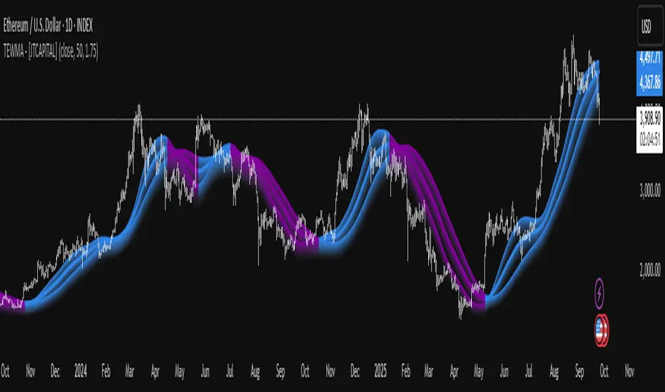
TEWMA - [JTCAPITAL]TEWMA - is a modified way to use Triple Exponential Moving Average (TEMA) combined with Weighted Moving Average (WMA) and adaptive multi-length averaging for Trend-Following.
The indicator blends short- and extended-length smoothed signals into a single adaptive line, then assigns directional bias to highlight bullish or bearish phases more clearly.
The indicator works by calculating in the following steps:
Source Selection
The script begins with a selectable price source (default: Close, but can be changed to Open, High, Low, HL2, etc.). This ensures flexibility depending on the user’s preferred market perspective.
Dual-Length Calculation
A base length ( len ) is chosen, and then multiplied by a factor ( multi , default 1.75). This produces a secondary, longer period ( len2 ) that adapts proportionally to the base.
Weighted + Triple Exponential Smoothing
-First, a WMA (Weighted Moving Average) is applied to the price source.
-Then, the TEMA (Triple Exponential Moving Average) is applied to smooth the WMA even further.
-This process is repeated for both len and len2 , producing TEWMA1 and TEWMA2 .
Adaptive Averaging
The final TEWMA line is calculated as the average of TEWMA1 and TEWMA2, creating a blend between the short-term and extended-term signals. This balances reactivity and stability, reducing lag while avoiding excessive noise.
Trend Direction Detection
-If TEWMA is greater than its previous value → Bullish .
-If TEWMA is lower than its previous value → Bearish .
-A Signal variable is used to store this directional bias, ensuring continuity between bars.
Visual Plotting
-The main TEWMA is plotted with bold coloring (Blue for bullish, Purple for bearish).
-TEWMA1 and TEWMA2 are plotted as thinner supporting lines.
-Each line is given a shadow-fill (between 100% and 90% of its value) for emphasis and visual clarity.
Alerts
Custom alerts are defined:
- TEWMA Long → when bullish.
- TEWMA Short → when bearish.
-These alerts can be integrated into TradingView’s alerting system for automated notifications.
Buy and Sell Conditions :
- Buy : Triggered when TEWMA rises (bullish slope). The indicator colors the line blue and an alert can be fired.
- Sell : Triggered when TEWMA declines (bearish slope). The line turns purple, signaling potential short or exit points.
Features and Parameters :
- Source → Selectable price input (Close, Open, HL2, etc.).
- Length (len) → Base period for the WMA/TEMA calculation.
- Multiplier (multi) → Scales the secondary length to create a longer-term smoothing.
- Color-coded Trend Lines → Blue for bullish, Purple for bearish.
- Shadow Fill Effects → Provides depth and easier visualization of trend direction.
- Alert Conditions → Prebuilt alerts for both Long and Short scenarios.
Specifications :
Weighted Moving Average (WMA)
The WMA assigns more weight to recent price values, making it more responsive than a Simple Moving Average (SMA). This enhances early detection of market turns while reducing lag compared to longer-term averages.
Triple Exponential Moving Average (TEMA)
TEMA is designed to minimize lag by combining multiple EMA layers (EMA of EMA of EMA). It is smoother and more adaptive than traditional EMAs, making it ideal for detecting true market direction without overreacting to small fluctuations.
Multi-Length Averaging
By calculating two versions of WMA → TEMA with different lengths and then averaging them, the indicator balances responsiveness (short-term sensitivity) and reliability (long-term confirmation). This prevents whipsawing while keeping signals timely.
Adaptive Signal Assignment
Instead of simply flipping signals at crossovers, the indicator checks slope direction of TEWMA. This ensures smoother trend-following behavior, reducing false positives in sideways conditions.
Color-Coding & Visual Shading
Visual clarity is achieved by coloring bullish periods differently from bearish ones, with shaded fills beneath each line. This allows traders to instantly identify trend conditions and compare short- vs long-term signals.
Alert Conditions
Trading decisions can be automated by attaching alerts to the TEWMA’s bullish and bearish states. This makes it practical for active trading, swing setups, or algorithmic strategies.
Enjoy!
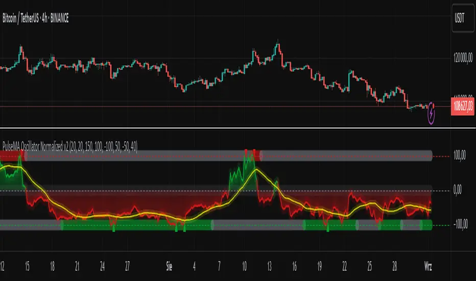
PulseMA Oscillator Normalized v2█ OVERVIEW
PulseMA Oscillator Normalized v2 is a technical indicator designed for the TradingView platform, assisting traders in identifying potential trend reversal points based on price dynamics derived from moving averages. The indicator is normalized for easier interpretation across various market conditions, and its visual presentation with gradients and signals facilitates quick decision-making.
█ CONCEPTS
The core idea of the indicator is to analyze trend dynamics by calculating an oscillator based on a moving average (EMA), which is then normalized and smoothed. It provides insights into trend strength, overbought/oversold levels, and reversal signals, enhanced by gradient visualizations.
Why use it?
Identifying reversal points: The indicator detects overbought and oversold levels, generating buy/sell signals at their crossovers.
Price dynamics analysis: Based on moving averages, it measures how long the price stays above or below the EMA, incorporating trend slope.
Visual clarity: Gradients, fills, and colored lines enable quick chart analysis.
Flexibility: Configurable parameters, such as moving average lengths or normalization period, allow adaptation to various strategies and markets.
How it works?
Trend detection: Calculates a base exponential moving average (EMA with PulseMA Length) and measures how long the price stays above or below it, multiplied by the slope for the oscillator.
Normalization: The oscillator is normalized based on the minimum and maximum values over a lookback period (default 150 bars), scaling it to a range from -100 to 100: (oscillator - min) / (max - min) * 200 - 100. This ensures values are comparable across different instruments and timeframes.
Smoothing: The main line (PulseMA) is the normalized oscillator (oscillatorNorm). The PulseMA MA line is a smoothed version of PulseMA, calculated using an SMA with the PulseMA MA length. As PulseMA MA is smoothed, it reacts more slowly and can be used as a noise filter.
Signals: Generates buy signals when crossing the oversold level upward and sell signals when crossing the overbought level downward. Signals are stronger when PulseMA MA is in the overbought or oversold zone (exceeding the respective thresholds for PulseMA MA).
Visualization: Draws lines with gradients for PulseMA and PulseMA MA, levels with gradients, gradient fill to the zero line, and signals as triangles.
Alerts: Built-in alerts for buy and sell signals.
Settings and customization
PulseMA Length: Length of the base EMA (default 20).
PulseMA MA: Length of the SMA for smoothing PulseMA MA (default 20).
Normalization Lookback Period: Normalization period (default 150, minimum 10).
Overbought/Oversold Levels: Levels for the main line (default 100/-100) and thresholds for PulseMA MA, indicating zones where PulseMA MA exceeds set values (default 50/-50).
Colors and gradients: Customize colors for lines, gradients, and levels; options to enable/disable gradients and fills.
Visualizations: Show PulseMA MA, gradients for overbought/oversold/zero levels, and fills.
█ OTHER SECTIONS
Usage examples
Trend analysis: Observe PulseMA above 0 for an uptrend or below 0 for a downtrend. Use different values for PulseMA Length and PulseMA MA to gain a clearer trend picture. PulseMA MA, being smoothed, reacts more slowly and can serve as a noise filter to confirm trend direction.
Reversal signals: Look for buy triangles when PulseMA crosses the oversold level, especially when PulseMA MA is in the oversold zone. Similarly, look for sell triangles when crossing the overbought level with PulseMA MA in the overbought zone. Such confirmation increases signal reliability.
Customization: Test different values for PulseMA Length and PulseMA MA on a given instrument and timeframe to minimize false signals and tailor the indicator to market specifics.
Notes for users
Combine with other tools, such as support/resistance levels or other oscillators, for greater accuracy.
Test different settings for PulseMA Length and PulseMA MA on the chosen instrument and timeframe to find optimal values.
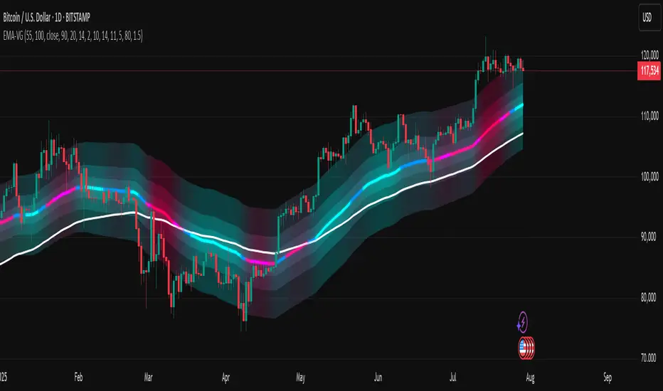
[LeonidasCrypto]EMA with Volatility GlowEMA Volatility Glow - Advanced Moving Average with Dynamic Volatility Visualization
Overview
The EMA Volatility Glow indicator combines dual exponential moving averages with a sophisticated volatility measurement system, enhanced by dynamic visual effects that respond to real-time market conditions.
Technical Components
Volatility Calculation Engine
BB Volatility Curve: Utilizes Bollinger Band width normalized through RSI smoothing
Multi-stage Noise Filtering: 3-layer exponential smoothing algorithm reduces market noise
Rate of Change Analysis: Dual-timeframe RoC calculation (14/11 periods) processed through weighted moving average
Dynamic Normalization: 100-period lookback for relative volatility assessment
Moving Average System
Primary EMA: Default 55-period exponential moving average with volatility-responsive coloring
Secondary EMA: Default 100-period exponential moving average for trend confirmation
Trend Analysis: Real-time bullish/bearish determination based on EMA crossover dynamics
Visual Enhancement Framework
Gradient Band System: Multi-layer volatility bands using Fibonacci ratios (0.236, 0.382, 0.618)
Dynamic Color Mapping: Five-tier color system reflecting volatility intensity levels
Configurable Glow Effects: Customizable transparency and intensity settings
Trend Fill Visualization: Directional bias indication between moving averages
Key Features
Volatility States:
Ultra-Low: Minimal market movement periods
Low: Reduced volatility environments
Medium: Normal market conditions
High: Increased volatility phases
Extreme: Exceptional market stress periods
Customization Options:
Adjustable EMA periods
Configurable glow intensity (1-10 levels)
Variable transparency controls
Toggleable visual components
Customizable gradient band width
Technical Calculations:
ATR-based gradient bands with noise filtering
ChartPrime-inspired multi-layer fill system
Real-time volatility curve computation
Smooth color gradient transitions
Applications
Trend Identification: Dual EMA system for directional bias assessment
Volatility Analysis: Real-time market stress evaluation
Risk Management: Visual volatility cues for position sizing decisions
Market Timing: Enhanced visual feedback for entry/exit consideration
PulseMA + MADescription
The PulseMA + MA indicator is an analytical tool that combines the analysis of the price relationship to a base Exponential Moving Average (EMA) with a smoothed Simple Moving Average (SMA) of this relationship. The indicator helps traders identify the direction and momentum of market trends and generates entry signals, displaying data as lines below the price chart.
Key Features
PulseMA: Calculates trend momentum by multiplying the number of consecutive candles above or below the base EMA by the slope of this average. The number of candles determines trend strength (positive for an uptrend, negative for a downtrend), while the EMA slope reflects the rate of change of the average. The PulseMA value is scaled by multiplying by 100.
Smoothed Average (PulseMA MA): Adds a smoothed SMA, facilitating the identification of long-term changes in market momentum.
Dynamic Colors: The PulseMA line changes color based on the price position relative to the base EMA (green for price above, red for price below).
Zero Line: Indicates the area where the price is close to the base EMA.
Applications
The PulseMA + MA indicator is designed for traders and technical analysts who aim to:
Analyze the direction and momentum of market trends, particularly with higher PulseMA Length values (e.g., 100), which provide a less sensitive EMA for longer-term trends.
Generate entry signals based on the PulseMA color change or the crossover of PulseMA with PulseMA MA.
Anticipate potential price reversals to the zero line when PulseMA is significantly distant from it, which may indicate market overextension.
How to Use
Add the Indicator to the Chart: Search for "PulseMA + MA" in the indicator library and add it to your chart.
Adjust Parameters:
PulseMA Length: Length of the base EMA (default: 50).
PulseMA Smoothing Length: Length of the smoothed SMA (default: 20).
Interpretation:
Green PulseMA Line: Price is above the base EMA, suggesting an uptrend.
Red PulseMA Line: Price is below the base EMA, indicating a downtrend.
PulseMA Color Change: May signal an entry point (recommended to wait for 2 candles to reduce noise).
PulseMA Crossing PulseMA MA from Below: May indicate a buy signal in an uptrend.
Zero Line: Indicates the area where the price is close to the base EMA.
Significant Deviation of PulseMA from the Zero Line: Suggests a potential price reversal to the zero line, indicating possible market overextension.
Notes
The indicator generates trend signals and can be used to independently identify entry points, e.g., on PulseMA color changes (waiting 2 candles is recommended to reduce noise) or when PulseMA crosses PulseMA MA from below.
In sideways markets, it is advisable to use the indicator with a volatility filter to limit false signals.
Adjusting the lengths of the averages to suit the specific instrument can improve signal accuracy.

PhenLabs - Market Fluid Dynamics📊 Market Fluid Dynamics -
Version: PineScript™ v6
📌 Description
The Market Fluid Dynamics - Phen indicator is a new thinking regarding market analysis by modeling price action, volume, and volatility using a fluid system. It attempts to offer traders control over more profound market forces, such as momentum (speed), resistance (thickness), and buying/selling pressure. By visualizing such dynamics, the script allows the traders to decide on the prevailing market flow, its power, likely continuations, and zones of calmness and chaos, and thereby allows improved decision-making.
This measure avoids the usual difficulty of reconciling multiple, often contradictory, market indications by including them within a single overarching model. It moves beyond traditional binary indicators by providing a multi-dimensional view of market behavior, employing fluid dynamic analogs to describe complex interactions in an accessible manner.
🚀 Points of Innovation
Integrated Fluid Dynamics Model: Combines velocity, viscosity, pressure, and turbulence into a single indicator.
Normalized Metrics: Uses ATR and other normalization techniques for consistent readings across different assets and timeframes.
Dynamic Flow Visualization: Main flow line changes color and intensity based on direction and strength.
Turbulence Background: Visually represents market stability with a gradient background, from calm to turbulent.
Comprehensive Dashboard: Provides an at-a-glance summary of key fluid dynamic metrics.
Multi-Layer Smoothing: Employs several layers of EMA smoothing for a clearer, more responsive main flow line.
🔧 Core Components
Velocity Component: Measures price momentum (first derivative of price), normalized by ATR. It indicates the speed and direction of price changes.
Viscosity Component: Represents market resistance to price changes, derived from ATR relative to its historical average. Higher viscosity suggests it’s harder for prices to move.
Pressure Component: Quantifies the force created by volume and price range (close - open), normalized by ATR. It reflects buying or selling pressure.
Turbulence Detection: Calculates a Reynolds number equivalent to identify market stability, ranging from laminar (stable) to turbulent (chaotic).
Main Flow Indicator: Combines the above components, applying sensitivity and smoothing, to generate a primary signal of market direction and strength.
🔥 Key Features
Advanced Smoothing Algorithm: Utilizes multiple EMA layers on the raw flow calculation for a fluid and responsive main flow line, reducing noise while maintaining sensitivity.
Gradient Flow Coloring: The main flow line dynamically changes color from light to deep blue for bullish flow and light to deep red for bearish flow, with intensity reflecting flow strength. This provides an immediate visual cue of market sentiment and momentum.
Turbulence Level Background: The chart background changes color based on calculated turbulence (from calm gray to vibrant orange), offering an intuitive understanding of market stability and potential for erratic price action.
Informative Dashboard: A customizable on-screen table displays critical metrics like Flow State, Flow Strength, Market Viscosity, Turbulence, Pressure Force, Flow Acceleration, and Flow Continuity, allowing traders to quickly assess current market conditions.
Configurable Lookback and Sensitivity: Users can adjust the base lookback period for calculations and the sensitivity of the flow to viscosity, tailoring the indicator to different trading styles and market conditions.
Alert Conditions: Pre-defined alerts for flow direction changes (positive/negative crossover of zero line) and detection of high turbulence states.
🎨 Visualization
Main Flow Line: A smoothed line plotted below the main chart, colored blue for bullish flow and red for bearish flow. The intensity of the color (light to dark) indicates the strength of the flow. This line crossing the zero line can signal a change in market direction.
Zero Line: A dotted horizontal line at the zero level, serving as a baseline to gauge whether the market flow is positive (bullish) or negative (bearish).
Turbulence Background: The indicator pane’s background color changes based on the calculated turbulence level. A calm, almost transparent gray indicates low turbulence (laminar flow), while a more vibrant, semi-transparent orange signifies high turbulence. This helps traders visually assess market stability.
Dashboard Table: An optional table displayed on the chart, showing key metrics like ‘Flow State’, ‘Flow Strength’, ‘Market Viscosity’, ‘Turbulence’, ‘Pressure Force’, ‘Flow Acceleration’, and ‘Flow Continuity’ with their current values and qualitative descriptions (e.g., ‘Bullish Flow’, ‘Laminar (Stable)’).
📖 Usage Guidelines
Setting Categories
Show Dashboard - Default: true; Range: true/false; Description: Toggles the visibility of the Market Fluid Dynamics dashboard on the chart. Enable to see key metrics at a glance.
Base Lookback Period - Default: 14; Range: 5 - (no upper limit, practical limits apply); Description: Sets the primary lookback period for core calculations like velocity, ATR, and volume SMA. Shorter periods make the indicator more sensitive to recent price action, while longer periods provide a smoother, slower signal.
Flow Sensitivity - Default: 0.5; Range: 0.1 - 1.0 (step 0.1); Description: Adjusts how much the market viscosity dampens the raw flow. A lower value means viscosity has less impact (flow is more sensitive to raw velocity/pressure), while a higher value means viscosity has a greater dampening effect.
Flow Smoothing - Default: 5; Range: 1 - 20; Description: Controls the length of the EMA smoothing applied to the main flow line. Higher values result in a smoother flow line but with more lag; lower values make it more responsive but potentially noisier.
Dashboard Position - Default: ‘Top Right’; Range: ‘Top Right’, ‘Top Left’, ‘Bottom Right’, ‘Bottom Left’, ‘Middle Right’, ‘Middle Left’; Description: Determines the placement of the dashboard on the chart.
Header Size - Default: ‘Normal’; Range: ‘Tiny’, ‘Small’, ‘Normal’, ‘Large’, ‘Huge’; Description: Sets the text size for the dashboard header.
Values Size - Default: ‘Small’; Range: ‘Tiny’, ‘Small’, ‘Normal’, ‘Large’; Description: Sets the text size for the metric values in the dashboard.
✅ Best Use Cases
Trend Identification: Identifying the dominant market flow (bullish or bearish) and its strength to trade in the direction of the prevailing trend.
Momentum Confirmation: Using the flow strength and acceleration to confirm the conviction behind price movements.
Volatility Assessment: Utilizing the turbulence metric to gauge market stability, helping to adjust position sizing or avoid choppy conditions.
Reversal Spotting: Watching for divergences between price and flow, or crossovers of the main flow line above/below the zero line, as potential reversal signals, especially when combined with changes in pressure or viscosity.
Swing Trading: Leveraging the smoothed flow line to capture medium-term market swings, entering when flow aligns with the desired trade direction and exiting when flow weakens or reverses.
Intraday Scalping: Using shorter lookback periods and higher sensitivity to identify quick shifts in flow and turbulence for short-term trading opportunities, particularly in liquid markets.
⚠️ Limitations
Lagging Nature: Like many indicators based on moving averages and lookback periods, the main flow line can lag behind rapid price changes, potentially leading to delayed signals.
Whipsaws in Ranging Markets: During periods of low volatility or sideways price action (high viscosity, low flow strength), the indicator might produce frequent buy/sell signals (whipsaws) as the flow oscillates around the zero line.
Not a Standalone System: While comprehensive, it should be used in conjunction with other forms of analysis (e.g., price action, support/resistance levels, other indicators) and not as a sole basis for trading decisions.
Subjectivity in Interpretation: While the dashboard provides quantitative values, the interpretation of “strong” flow, “high” turbulence, or “significant” acceleration can still have a subjective element depending on the trader’s strategy and risk tolerance.
💡 What Makes This Unique
Fluid Dynamics Analogy: Its core strength lies in translating complex market interactions into an intuitive fluid dynamics framework, making concepts like momentum, resistance, and pressure easier to visualize and understand.
Market View: Instead of focusing on a single aspect (like just momentum or just volatility), it integrates multiple factors (velocity, viscosity, pressure, turbulence) to provide a more comprehensive picture of market conditions.
Adaptive Visualization: The dynamic coloring of the flow line and the turbulence background provide immediate, adaptive visual feedback that changes with market conditions.
🔬 How It Works
Price Velocity Calculation: The indicator first calculates price velocity by measuring the rate of change of the closing price over a given ‘lookback’ period. The raw velocity is then normalized by the Average True Range (ATR) of the same lookback period. Normalization enables comparison of momentum between assets or timeframes by scaling for volatility. This is the direction and speed of initial price movement.
Viscosity Calculation: Market ‘viscosity’ or resistance to price movement is determined by looking at the current ATR relative to its longer-term average (SMA of ATR over lookback * 2). The further the current ATR is above its average, the lower the viscosity (less resistance to price movement), and vice-versa. The script inverts this relationship and bounds it so that rising viscosity means more resistance.
Pressure Force Measurement: A ‘pressure’ variable is calculated as a function of the ratio of current volume to its simple moving average, multiplied by the price range (close - open) and normalized by ATR. This is designed to measure the force behind price movement created by volume and intraday price thrusts. This pressure is smoothed by an EMA.
Turbulence State Evaluation: A equivalent ‘Reynolds number’ is calculated by dividing the absolute normalized velocity by the viscosity. This is the proclivity of the market to move in a chaotic or orderly fashion. This ‘reynoldsValue’ is smoothed with an EMA to get the ‘turbulenceState’, which indicates if the market is laminar (stable), transitional, or turbulent.
Main Flow Derivation: The ‘rawFlow’ is calculated by taking the normalized velocity, dampening its impact based on the ‘viscosity’ and user-input ‘sensitivity’, and orienting it by the sign of the smoothed ‘pressureSmooth’. The ‘rawFlow’ is then put through multiple layers of exponential moving average (EMA) smoothing (with ‘smoothingLength’ and derived values) to reach the final ‘mainFlow’ line. The extensive smoothing is designed to give a smooth and clear visualization of the overall market direction and magnitude.
Dashboard Metrics Compilation: Additional metrics like flow acceleration (derivative of mainFlow), and flow continuity (correlation between close and volume) are calculated. All primary components (Flow State, Strength, Viscosity, Turbulence, Pressure, Acceleration, Continuity) are then presented in a user-configurable dashboard for ease of monitoring.
💡 Note:
The “Market Fluid Dynamics - Phen” indicator is designed to offer a unique perspective on market behavior by applying principles from fluid dynamics. It’s most effective when used to understand the underlying forces driving price rather than as a direct buy/sell signal generator in isolation. Experiment with the settings, particularly the ‘Base Lookback Period’, ‘Flow Sensitivity’, and ‘Flow Smoothing’, to find what best suits your trading style and the specific asset you are analyzing. Always combine its insights with robust risk management practices.
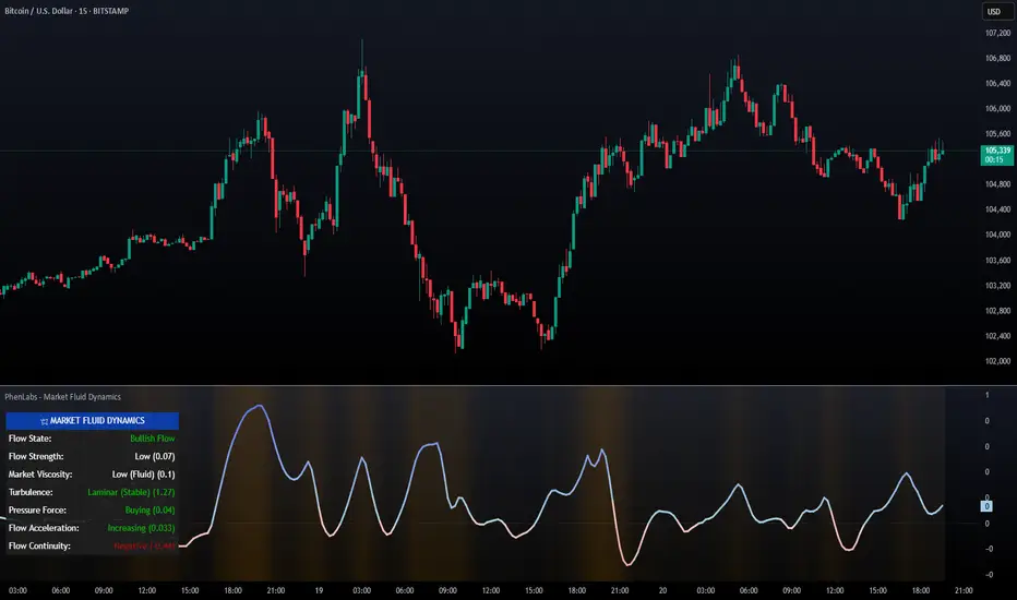
CAN INDICATORCAN Moving Averages Indicator - Feature Guide
1. Multiple Moving Averages (20 MAs)
- Supports up to 20 individual moving averages
- Each MA can be independently configured:
- Enable/Disable toggle
- Length (period) setting
- Type selection (SMA, EMA, DEMA, VWMA, RMA, WMA)
- Color customization
- Individual timeframe settings when global timeframe is disabled
Pre-configured MA Settings:
1. MA1-8: SMA type
- Lengths: 20, 50, 100, 200, 365, 489, 600, 1460
2. MA9-20: EMA type
- Lengths: 30, 60, 120, 240, 300, 400, 500, 700, 800, 900, 1000, 2000
2. Global Timeframe Settings
Location: Global Settings group
Features:
- Use Global Timeframe: Toggle to use one timeframe for all MAs
- Global Timeframe: Select the timeframe to apply globally
3. Label Display Options
Location: Main Inputs section
Controls:
- Show MA Type: Display MA type (SMA, EMA, etc.)
- Show MA Length: Display period length
- Show Resolution: Display timeframe
- Label Offset: Adjust label position
4. Cross Alerts System
Location: Cross Alerts group
Features:
1. Price Crosses:
- Alerts when price crosses any selected MA
- Select MA to monitor (1-20)
- Triggers on crossover/crossunder
2. MA Crosses:
- Alerts when one MA crosses another
- Select fast MA (1-20)
- Select slow MA (1-20)
- Triggers on crossover/crossunder
5. Relative Strength (RS) Analysis
Location: Relative Strength group
Features:
- Select any MA to monitor (1-20)
- Compares MA to its own average
- Adjustable RS Length (default 14)
- Visual feedback via background color:
- Green: MA above its average (uptrend)
- Red: MA below its average (downtrend)
- Customizable colors and transparency
6. Moving Average Types Available
1. **SMA** (Simple Moving Average)
- Equal weight to all prices
2. **EMA** (Exponential Moving Average)
- More weight to recent prices
3. **DEMA** (Double Exponential Moving Average)
- Reduced lag compared to EMA
4. **VWMA** (Volume Weighted Moving Average)
- Incorporates volume data
5. **RMA** (Running Moving Average)
- Smoother than EMA
6. **WMA** (Weighted Moving Average)
- Linear weight distribution
Usage Tips
1. **For Trend Following:**
- Enable longer-period MAs (MA4-MA8)
- Use cross alerts between long-term MAs
- Monitor RS for trend strength
2. **For Short-term Trading:**
- Focus on shorter-period MAs (MA1-MA3, MA9-MA11)
- Enable price cross alerts
- Use multiple timeframe analysis
3. **For Multiple Timeframe Analysis:**
- Disable global timeframe
- Set different timeframes for each MA
- Compare MA relationships across timeframes
4. **For Performance:**
- Disable unused MAs
- Limit active alerts to necessary pairs
- Use RS selectively on key MAs

real_time_candlesIntroduction
The Real-Time Candles Library provides comprehensive tools for creating, manipulating, and visualizing custom timeframe candles in Pine Script. Unlike standard indicators that only update at bar close, this library enables real-time visualization of price action and indicators within the current bar, offering traders unprecedented insight into market dynamics as they unfold.
This library addresses a fundamental limitation in traditional technical analysis: the inability to see how indicators evolve between bar closes. By implementing sophisticated real-time data processing techniques, traders can now observe indicator movements, divergences, and trend changes as they develop, potentially identifying trading opportunities much earlier than with conventional approaches.
Key Features
The library supports two primary candle generation approaches:
Chart-Time Candles: Generate real-time OHLC data for any variable (like RSI, MACD, etc.) while maintaining synchronization with chart bars.
Custom Timeframe (CTF) Candles: Create candles with custom time intervals or tick counts completely independent of the chart's native timeframe.
Both approaches support traditional candlestick and Heikin-Ashi visualization styles, with options for moving average overlays to smooth the data.
Configuration Requirements
For optimal performance with this library:
Set max_bars_back = 5000 in your script settings
When using CTF drawing functions, set max_lines_count = 500, max_boxes_count = 500, and max_labels_count = 500
These settings ensure that you will be able to draw correctly and will avoid any runtime errors.
Usage Examples
Basic Chart-Time Candle Visualization
// Create real-time candles for RSI
float rsi = ta.rsi(close, 14)
Candle rsi_candle = candle_series(rsi, CandleType.candlestick)
// Plot the candles using Pine's built-in function
plotcandle(rsi_candle.Open, rsi_candle.High, rsi_candle.Low, rsi_candle.Close,
"RSI Candles", rsi_candle.candle_color, rsi_candle.candle_color)
Multiple Access Patterns
The library provides three ways to access candle data, accommodating different programming styles:
// 1. Array-based access for collection operations
Candle candles = candle_array(source)
// 2. Object-oriented access for single entity manipulation
Candle candle = candle_series(source)
float value = candle.source(Source.HLC3)
// 3. Tuple-based access for functional programming styles
= candle_tuple(source)
Custom Timeframe Examples
// Create 20-second candles with EMA overlay
plot_ctf_candles(
source = close,
candle_type = CandleType.candlestick,
sample_type = SampleType.Time,
number_of_seconds = 20,
timezone = -5,
tied_open = true,
ema_period = 9,
enable_ema = true
)
// Create tick-based candles (new candle every 15 ticks)
plot_ctf_tick_candles(
source = close,
candle_type = CandleType.heikin_ashi,
number_of_ticks = 15,
timezone = -5,
tied_open = true
)
Advanced Usage with Custom Visualization
// Get custom timeframe candles without automatic plotting
CandleCTF my_candles = ctf_candles_array(
source = close,
candle_type = CandleType.candlestick,
sample_type = SampleType.Time,
number_of_seconds = 30
)
// Apply custom logic to the candles
float ema_values = my_candles.ctf_ema(14)
// Draw candles and EMA using time-based coordinates
my_candles.draw_ctf_candles_time()
ema_values.draw_ctf_line_time(line_color = #FF6D00)
Library Components
Data Types
Candle: Structure representing chart-time candles with OHLC, polarity, and visualization properties
CandleCTF: Extended candle structure with additional time metadata for custom timeframes
TickData: Structure for individual price updates with time deltas
Enumerations
CandleType: Specifies visualization style (candlestick or Heikin-Ashi)
Source: Defines price components for calculations (Open, High, Low, Close, HL2, etc.)
SampleType: Sets sampling method (Time-based or Tick-based)
Core Functions
get_tick(): Captures current price as a tick data point
candle_array(): Creates an array of candles from price updates
candle_series(): Provides a single candle based on latest data
candle_tuple(): Returns OHLC values as a tuple
ctf_candles_array(): Creates custom timeframe candles without rendering
Visualization Functions
source(): Extracts specific price components from candles
candle_ctf_to_float(): Converts candle data to float arrays
ctf_ema(): Calculates exponential moving averages for candle arrays
draw_ctf_candles_time(): Renders candles using time coordinates
draw_ctf_candles_index(): Renders candles using bar index coordinates
draw_ctf_line_time(): Renders lines using time coordinates
draw_ctf_line_index(): Renders lines using bar index coordinates
Technical Implementation Notes
This library leverages Pine Script's varip variables for state management, creating a sophisticated real-time data processing system. The implementation includes:
Efficient tick capturing: Samples price at every execution, maintaining temporal tracking with time deltas
Smart state management: Uses a hybrid approach with mutable updates at index 0 and historical preservation at index 1+
Temporal synchronization: Manages two time domains (chart time and custom timeframe)
The tooltip implementation provides crucial temporal context for custom timeframe visualizations, allowing users to understand exactly when each candle formed regardless of chart timeframe.
Limitations
Custom timeframe candles cannot be backtested due to Pine Script's limitations with historical tick data
Real-time visualization is only available during live chart updates
Maximum history is constrained by Pine Script's array size limits
Applications
Indicator visualization: See how RSI, MACD, or other indicators evolve in real-time
Volume analysis: Create custom volume profiles independent of chart timeframe
Scalping strategies: Identify short-term patterns with precisely defined time windows
Volatility measurement: Track price movement characteristics within bars
Custom signal generation: Create entry/exit signals based on custom timeframe patterns
Conclusion
The Real-Time Candles Library bridges the gap between traditional technical analysis (based on discrete OHLC bars) and the continuous nature of market movement. By making indicators more responsive to real-time price action, it gives traders a significant edge in timing and decision-making, particularly in fast-moving markets where waiting for bar close could mean missing important opportunities.
Whether you're building custom indicators, researching price patterns, or developing trading strategies, this library provides the foundation for sophisticated real-time analysis in Pine Script.
Implementation Details & Advanced Guide
Core Implementation Concepts
The Real-Time Candles Library implements a sophisticated event-driven architecture within Pine Script's constraints. At its heart, the library creates what's essentially a reactive programming framework handling continuous data streams.
Tick Processing System
The foundation of the library is the get_tick() function, which captures price updates as they occur:
export get_tick(series float source = close, series float na_replace = na)=>
varip float price = na
varip int series_index = -1
varip int old_time = 0
varip int new_time = na
varip float time_delta = 0
// ...
This function:
Samples the current price
Calculates time elapsed since last update
Maintains a sequential index to track updates
The resulting TickData structure serves as the fundamental building block for all candle generation.
State Management Architecture
The library employs a sophisticated state management system using varip variables, which persist across executions within the same bar. This creates a hybrid programming paradigm that's different from standard Pine Script's bar-by-bar model.
For chart-time candles, the core state transition logic is:
// Real-time update of current candle
candle_data := Candle.new(Open, High, Low, Close, polarity, series_index, candle_color)
candles.set(0, candle_data)
// When a new bar starts, preserve the previous candle
if clear_state
candles.insert(1, candle_data)
price.clear()
// Reset state for new candle
Open := Close
price.push(Open)
series_index += 1
This pattern of updating index 0 in real-time while inserting completed candles at index 1 creates an elegant solution for maintaining both current state and historical data.
Custom Timeframe Implementation
The custom timeframe system manages its own time boundaries independent of chart bars:
bool clear_state = switch settings.sample_type
SampleType.Ticks => cumulative_series_idx >= settings.number_of_ticks
SampleType.Time => cumulative_time_delta >= settings.number_of_seconds
This dual-clock system synchronizes two time domains:
Pine's execution clock (bar-by-bar processing)
The custom timeframe clock (tick or time-based)
The library carefully handles temporal discontinuities, ensuring candle formation remains accurate despite irregular tick arrival or market gaps.
Advanced Usage Techniques
1. Creating Custom Indicators with Real-Time Candles
To develop indicators that process real-time data within the current bar:
// Get real-time candles for your data
Candle rsi_candles = candle_array(ta.rsi(close, 14))
// Calculate indicator values based on candle properties
float signal = ta.ema(rsi_candles.first().source(Source.Close), 9)
// Detect patterns that occur within the bar
bool divergence = close > close and rsi_candles.first().Close < rsi_candles.get(1).Close
2. Working with Custom Timeframes and Plotting
For maximum flexibility when visualizing custom timeframe data:
// Create custom timeframe candles
CandleCTF volume_candles = ctf_candles_array(
source = volume,
candle_type = CandleType.candlestick,
sample_type = SampleType.Time,
number_of_seconds = 60
)
// Convert specific candle properties to float arrays
float volume_closes = volume_candles.candle_ctf_to_float(Source.Close)
// Calculate derived values
float volume_ema = volume_candles.ctf_ema(14)
// Create custom visualization
volume_candles.draw_ctf_candles_time()
volume_ema.draw_ctf_line_time(line_color = color.orange)
3. Creating Hybrid Timeframe Analysis
One powerful application is comparing indicators across multiple timeframes:
// Standard chart timeframe RSI
float chart_rsi = ta.rsi(close, 14)
// Custom 5-second timeframe RSI
CandleCTF ctf_candles = ctf_candles_array(
source = close,
candle_type = CandleType.candlestick,
sample_type = SampleType.Time,
number_of_seconds = 5
)
float fast_rsi_array = ctf_candles.candle_ctf_to_float(Source.Close)
float fast_rsi = fast_rsi_array.first()
// Generate signals based on divergence between timeframes
bool entry_signal = chart_rsi < 30 and fast_rsi > fast_rsi_array.get(1)
Final Notes
This library represents an advanced implementation of real-time data processing within Pine Script's constraints. By creating a reactive programming framework for handling continuous data streams, it enables sophisticated analysis typically only available in dedicated trading platforms.
The design principles employed—including state management, temporal processing, and object-oriented architecture—can serve as patterns for other advanced Pine Script development beyond this specific application.
------------------------
Library "real_time_candles"
A comprehensive library for creating real-time candles with customizable timeframes and sampling methods.
Supports both chart-time and custom-time candles with options for candlestick and Heikin-Ashi visualization.
Allows for tick-based or time-based sampling with moving average overlay capabilities.
get_tick(source, na_replace)
Captures the current price as a tick data point
Parameters:
source (float) : Optional - Price source to sample (defaults to close)
na_replace (float) : Optional - Value to use when source is na
Returns: TickData structure containing price, time since last update, and sequential index
candle_array(source, candle_type, sync_start, bullish_color, bearish_color)
Creates an array of candles based on price updates
Parameters:
source (float) : Optional - Price source to sample (defaults to close)
candle_type (simple CandleType) : Optional - Type of candle chart to create (candlestick or Heikin-Ashi)
sync_start (simple bool) : Optional - Whether to synchronize with the start of a new bar
bullish_color (color) : Optional - Color for bullish candles
bearish_color (color) : Optional - Color for bearish candles
Returns: Array of Candle objects ordered with most recent at index 0
candle_series(source, candle_type, wait_for_sync, bullish_color, bearish_color)
Provides a single candle based on the latest price data
Parameters:
source (float) : Optional - Price source to sample (defaults to close)
candle_type (simple CandleType) : Optional - Type of candle chart to create (candlestick or Heikin-Ashi)
wait_for_sync (simple bool) : Optional - Whether to wait for a new bar before starting
bullish_color (color) : Optional - Color for bullish candles
bearish_color (color) : Optional - Color for bearish candles
Returns: A single Candle object representing the current state
candle_tuple(source, candle_type, wait_for_sync, bullish_color, bearish_color)
Provides candle data as a tuple of OHLC values
Parameters:
source (float) : Optional - Price source to sample (defaults to close)
candle_type (simple CandleType) : Optional - Type of candle chart to create (candlestick or Heikin-Ashi)
wait_for_sync (simple bool) : Optional - Whether to wait for a new bar before starting
bullish_color (color) : Optional - Color for bullish candles
bearish_color (color) : Optional - Color for bearish candles
Returns: Tuple representing current candle values
method source(self, source, na_replace)
Extracts a specific price component from a Candle
Namespace types: Candle
Parameters:
self (Candle)
source (series Source) : Type of price data to extract (Open, High, Low, Close, or composite values)
na_replace (float) : Optional - Value to use when source value is na
Returns: The requested price value from the candle
method source(self, source)
Extracts a specific price component from a CandleCTF
Namespace types: CandleCTF
Parameters:
self (CandleCTF)
source (simple Source) : Type of price data to extract (Open, High, Low, Close, or composite values)
Returns: The requested price value from the candle as a varip
method candle_ctf_to_float(self, source)
Converts a specific price component from each CandleCTF to a float array
Namespace types: array
Parameters:
self (array)
source (simple Source) : Optional - Type of price data to extract (defaults to Close)
Returns: Array of float values extracted from the candles, ordered with most recent at index 0
method ctf_ema(self, ema_period)
Calculates an Exponential Moving Average for a CandleCTF array
Namespace types: array
Parameters:
self (array)
ema_period (simple float) : Period for the EMA calculation
Returns: Array of float values representing the EMA of the candle data, ordered with most recent at index 0
method draw_ctf_candles_time(self, sample_type, number_of_ticks, number_of_seconds, timezone)
Renders custom timeframe candles using bar time coordinates
Namespace types: array
Parameters:
self (array)
sample_type (simple SampleType) : Optional - Method for sampling data (Time or Ticks), used for tooltips
number_of_ticks (simple int) : Optional - Number of ticks per candle (used when sample_type is Ticks), used for tooltips
number_of_seconds (simple float) : Optional - Time duration per candle in seconds (used when sample_type is Time), used for tooltips
timezone (simple int) : Optional - Timezone offset from UTC (-12 to +12), used for tooltips
Returns: void - Renders candles on the chart using time-based x-coordinates
method draw_ctf_candles_index(self, sample_type, number_of_ticks, number_of_seconds, timezone)
Renders custom timeframe candles using bar index coordinates
Namespace types: array
Parameters:
self (array)
sample_type (simple SampleType) : Optional - Method for sampling data (Time or Ticks), used for tooltips
number_of_ticks (simple int) : Optional - Number of ticks per candle (used when sample_type is Ticks), used for tooltips
number_of_seconds (simple float) : Optional - Time duration per candle in seconds (used when sample_type is Time), used for tooltips
timezone (simple int) : Optional - Timezone offset from UTC (-12 to +12), used for tooltips
Returns: void - Renders candles on the chart using index-based x-coordinates
method draw_ctf_line_time(self, source, line_size, line_color)
Renders a line representing a price component from the candles using time coordinates
Namespace types: array
Parameters:
self (array)
source (simple Source) : Optional - Type of price data to extract (defaults to Close)
line_size (simple int) : Optional - Width of the line
line_color (simple color) : Optional - Color of the line
Returns: void - Renders a connected line on the chart using time-based x-coordinates
method draw_ctf_line_time(self, line_size, line_color)
Renders a line from a varip float array using time coordinates
Namespace types: array
Parameters:
self (array)
line_size (simple int) : Optional - Width of the line, defaults to 2
line_color (simple color) : Optional - Color of the line
Returns: void - Renders a connected line on the chart using time-based x-coordinates
method draw_ctf_line_index(self, source, line_size, line_color)
Renders a line representing a price component from the candles using index coordinates
Namespace types: array
Parameters:
self (array)
source (simple Source) : Optional - Type of price data to extract (defaults to Close)
line_size (simple int) : Optional - Width of the line
line_color (simple color) : Optional - Color of the line
Returns: void - Renders a connected line on the chart using index-based x-coordinates
method draw_ctf_line_index(self, line_size, line_color)
Renders a line from a varip float array using index coordinates
Namespace types: array
Parameters:
self (array)
line_size (simple int) : Optional - Width of the line, defaults to 2
line_color (simple color) : Optional - Color of the line
Returns: void - Renders a connected line on the chart using index-based x-coordinates
plot_ctf_tick_candles(source, candle_type, number_of_ticks, timezone, tied_open, ema_period, bullish_color, bearish_color, line_width, ema_color, use_time_indexing)
Plots tick-based candles with moving average
Parameters:
source (float) : Input price source to sample
candle_type (simple CandleType) : Type of candle chart to display
number_of_ticks (simple int) : Number of ticks per candle
timezone (simple int) : Timezone offset from UTC (-12 to +12)
tied_open (simple bool) : Whether to tie open price to close of previous candle
ema_period (simple float) : Period for the exponential moving average
bullish_color (color) : Optional - Color for bullish candles
bearish_color (color) : Optional - Color for bearish candles
line_width (simple int) : Optional - Width of the moving average line, defaults to 2
ema_color (color) : Optional - Color of the moving average line
use_time_indexing (simple bool) : Optional - When true the function will plot with xloc.time, when false it will plot using xloc.bar_index
Returns: void - Creates visual candle chart with EMA overlay
plot_ctf_tick_candles(source, candle_type, number_of_ticks, timezone, tied_open, bullish_color, bearish_color, use_time_indexing)
Plots tick-based candles without moving average
Parameters:
source (float) : Input price source to sample
candle_type (simple CandleType) : Type of candle chart to display
number_of_ticks (simple int) : Number of ticks per candle
timezone (simple int) : Timezone offset from UTC (-12 to +12)
tied_open (simple bool) : Whether to tie open price to close of previous candle
bullish_color (color) : Optional - Color for bullish candles
bearish_color (color) : Optional - Color for bearish candles
use_time_indexing (simple bool) : Optional - When true the function will plot with xloc.time, when false it will plot using xloc.bar_index
Returns: void - Creates visual candle chart without moving average
plot_ctf_time_candles(source, candle_type, number_of_seconds, timezone, tied_open, ema_period, bullish_color, bearish_color, line_width, ema_color, use_time_indexing)
Plots time-based candles with moving average
Parameters:
source (float) : Input price source to sample
candle_type (simple CandleType) : Type of candle chart to display
number_of_seconds (simple float) : Time duration per candle in seconds
timezone (simple int) : Timezone offset from UTC (-12 to +12)
tied_open (simple bool) : Whether to tie open price to close of previous candle
ema_period (simple float) : Period for the exponential moving average
bullish_color (color) : Optional - Color for bullish candles
bearish_color (color) : Optional - Color for bearish candles
line_width (simple int) : Optional - Width of the moving average line, defaults to 2
ema_color (color) : Optional - Color of the moving average line
use_time_indexing (simple bool) : Optional - When true the function will plot with xloc.time, when false it will plot using xloc.bar_index
Returns: void - Creates visual candle chart with EMA overlay
plot_ctf_time_candles(source, candle_type, number_of_seconds, timezone, tied_open, bullish_color, bearish_color, use_time_indexing)
Plots time-based candles without moving average
Parameters:
source (float) : Input price source to sample
candle_type (simple CandleType) : Type of candle chart to display
number_of_seconds (simple float) : Time duration per candle in seconds
timezone (simple int) : Timezone offset from UTC (-12 to +12)
tied_open (simple bool) : Whether to tie open price to close of previous candle
bullish_color (color) : Optional - Color for bullish candles
bearish_color (color) : Optional - Color for bearish candles
use_time_indexing (simple bool) : Optional - When true the function will plot with xloc.time, when false it will plot using xloc.bar_index
Returns: void - Creates visual candle chart without moving average
plot_ctf_candles(source, candle_type, sample_type, number_of_ticks, number_of_seconds, timezone, tied_open, ema_period, bullish_color, bearish_color, enable_ema, line_width, ema_color, use_time_indexing)
Unified function for plotting candles with comprehensive options
Parameters:
source (float) : Input price source to sample
candle_type (simple CandleType) : Optional - Type of candle chart to display
sample_type (simple SampleType) : Optional - Method for sampling data (Time or Ticks)
number_of_ticks (simple int) : Optional - Number of ticks per candle (used when sample_type is Ticks)
number_of_seconds (simple float) : Optional - Time duration per candle in seconds (used when sample_type is Time)
timezone (simple int) : Optional - Timezone offset from UTC (-12 to +12)
tied_open (simple bool) : Optional - Whether to tie open price to close of previous candle
ema_period (simple float) : Optional - Period for the exponential moving average
bullish_color (color) : Optional - Color for bullish candles
bearish_color (color) : Optional - Color for bearish candles
enable_ema (bool) : Optional - Whether to display the EMA overlay
line_width (simple int) : Optional - Width of the moving average line, defaults to 2
ema_color (color) : Optional - Color of the moving average line
use_time_indexing (simple bool) : Optional - When true the function will plot with xloc.time, when false it will plot using xloc.bar_index
Returns: void - Creates visual candle chart with optional EMA overlay
ctf_candles_array(source, candle_type, sample_type, number_of_ticks, number_of_seconds, tied_open, bullish_color, bearish_color)
Creates an array of custom timeframe candles without rendering them
Parameters:
source (float) : Input price source to sample
candle_type (simple CandleType) : Type of candle chart to create (candlestick or Heikin-Ashi)
sample_type (simple SampleType) : Method for sampling data (Time or Ticks)
number_of_ticks (simple int) : Optional - Number of ticks per candle (used when sample_type is Ticks)
number_of_seconds (simple float) : Optional - Time duration per candle in seconds (used when sample_type is Time)
tied_open (simple bool) : Optional - Whether to tie open price to close of previous candle
bullish_color (color) : Optional - Color for bullish candles
bearish_color (color) : Optional - Color for bearish candles
Returns: Array of CandleCTF objects ordered with most recent at index 0
Candle
Structure representing a complete candle with price data and display properties
Fields:
Open (series float) : Opening price of the candle
High (series float) : Highest price of the candle
Low (series float) : Lowest price of the candle
Close (series float) : Closing price of the candle
polarity (series bool) : Boolean indicating if candle is bullish (true) or bearish (false)
series_index (series int) : Sequential index identifying the candle in the series
candle_color (series color) : Color to use when rendering the candle
ready (series bool) : Boolean indicating if candle data is valid and ready for use
TickData
Structure for storing individual price updates
Fields:
price (series float) : The price value at this tick
time_delta (series float) : Time elapsed since the previous tick in milliseconds
series_index (series int) : Sequential index identifying this tick
CandleCTF
Structure representing a custom timeframe candle with additional time metadata
Fields:
Open (series float) : Opening price of the candle
High (series float) : Highest price of the candle
Low (series float) : Lowest price of the candle
Close (series float) : Closing price of the candle
polarity (series bool) : Boolean indicating if candle is bullish (true) or bearish (false)
series_index (series int) : Sequential index identifying the candle in the series
open_time (series int) : Timestamp marking when the candle was opened (in Unix time)
time_delta (series float) : Duration of the candle in milliseconds
candle_color (series color) : Color to use when rendering the candle

Smart Money Index + True Strength IndexThe Smart Money Index + True Strength Index indicator is a combination of two popular technical analysis indicators: the Smart Money Index (SMI) and the True Strength Index (TSI). This combined indicator helps traders identify potential entry points for long and short positions based on signals from both indexes.
Main Components:
Smart Money Index (SMI):
The SMI measures the difference between the closing and opening price of a candle multiplied by the trading volume over a certain period of time. This allows you to assess the activity of large players ("smart money") in the market. If the SMI value is above a certain threshold (smiThreshold), it may indicate a bullish trend, and if lower, it may indicate a bearish trend.
True Strength Index (TSI):
The TSI is an oscillator that measures the strength of a trend by comparing the price change of the current bar with the previous bar. It uses two exponential moving averages (EMAS) to smooth the data. TSI values can fluctuate around zero, with values above the overbought level indicating a possible downward correction, and values below the oversold level signaling a possible upward correction.
Parameters:
SMI Length: Defines the number of candles used to calculate the average SMI value. The default value is 14.
SMI Threshold: A threshold value that is used to determine a buy or sell signal. The default value is 0.
Length of the first TSI smoothing (tsiLength1): The length of the first EMA for calculating TSI. The default value is 25.
Second TSI smoothing length (tsiLength2): The length of the second EMA for additional smoothing of TSI values. The default value is 13.
TSI Overbought level: The level at which the market is considered to be overbought. The default value is 25.
Oversold level TSI: The level at which it is considered that the market is in an oversold state. The default value is -25.
Logic of operation:
SMI calculation:
First, the difference between the closing and opening price of each candle (close - open) is calculated.
This difference is then multiplied by the trading volume.
The resulting product is averaged using a simple moving average (SMA) over a specified period (smiLength).
Calculation of TSI:
The price change relative to the previous bar is calculated (close - close ).
The first EMA with the length tsiLength1 is applied.
Next, a second EMA with a length of tsiLength2 is applied to obtain the final TSI value.
The absolute value of price changes is calculated in the same way, and two emas are also applied.
The final TSI index is calculated as the ratio of these two values multiplied by 100.
Graphical representation:
The SMI and TSI lines are plotted on the graph along with their respective thresholds.
For SMI, the line is drawn in orange, and the threshold level is dotted in gray.
For the TSI, the line is plotted in blue, the overbought and oversold levels are indicated by red and green dotted lines, respectively.
Conditions for buy/sell signals:
A buy (long) signal is generated when:
SMI is greater than the threshold (smi > smiThreshold)
TSI crosses the oversold level from bottom to top (ta.crossover(tsi, oversold)).
A sell (short) signal is generated when:
SMI is less than the threshold (smi < smiThreshold)
TSI crosses the overbought level from top to bottom (ta.crossunder(tsi, overbought)).
Signal display:
When the conditions for a long or short are met, labels labeled "LONG" or "SHORT" appear on the chart.
The label for the long is located under the candle and is colored green, and for the short it is above the candle and is colored red.
Notification generation:
The indicator also supports notifications via the TradingView platform. Notifications are sent when conditions arise for a long or short position.
This combined indicator provides the trader with the opportunity to use both SMI and TSI signals simultaneously, which can improve the accuracy of trading decisions.
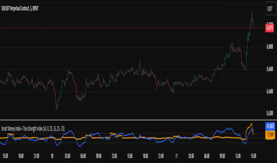
RoGr75 Adaptive EMA CrossDescription:
The RoGr75 Adaptive EMA Cross indicator dynamically combines exponential moving averages (EMAs) with ATR-based volatility buffers to generate buy and sell signals across multiple timeframes. This script uses customizable settings for short and long EMAs, ATR, and volume filters, ensuring that signals are both volatility-adjusted and timeframe-aware. It includes features such as adaptive buffers, distinct price level filters for buying and selling, and a reset mechanism to prevent redundant signals. Additionally, the indicator manages signal labels efficiently to keep your chart uncluttered.
Warning:
This script is provided for testing and educational purposes only. It is not intended as financial advice, and past performance does not guarantee future results. Use at your own risk. Always conduct your own research before making any trading decisions.
Higher Timeframe Input: Choose a specific timeframe for the indicator’s calculations; leave blank to use the chart’s current timeframe.
Signal Distance: Sets the distance of signal labels from the candles as a multiple of the ATR.
Exact Value Offset: Adjusts the secondary marker’s position for precision on the chart.
ATR Length: Defines the period used to calculate the Average True Range for volatility measurement.
EMA Lengths: Specify the periods for the short and long exponential moving averages.
Buy/Sell Buffer ATR Multipliers: Dynamically adjust the trigger distance beyond the EMA crossovers based on volatility.
Price Level Filter: Activates a filter so that buy signals only occur above a set price and sell signals only occur below that price (0 disables the filter).
Volume Filter: Optionally requires current volume to exceed a set multiple of a 20-period average for signal confirmation.
Reset Period: Resets the last signal memory after a specified number of bars to avoid suppressing valid repeat signals.
EMA Colors & Line Width: Customize the appearance of the short and long EMAs.
Label Colors & Styles: Choose colors, text colors, and styles for the buy and sell signal labels.
Background Highlighting: Optionally colors the background when a buy or sell signal occurs.
Label Management: Automatically removes the oldest labels when a set maximum is reached to keep the chart clean.
Alerts: Predefined conditions allow you to set TradingView alerts when buy or sell signals are generated.
Warning: This indicator is for testing purposes only and is not financial advice. Use it at your own risk.

Exponential Avg Body Size Green vs RedDescription :
This indicator calculates and plots the Exponential Moving Average (EMA) of green and red candlestick body sizes, allowing traders to easily visualize market momentum and sentiment shifts. The script includes the following features:
Customizable EMA Period: Users can set the number of candles to calculate the EMA through an input setting, with a default value of 21.
Separate Green and Red Candle Averages: Differentiates between bullish (green) and bearish (red) candlestick movements, plotting them as distinct lines.
Dynamic Range Control: Users can adjust the chart range (e.g., -50 to 50) for better visibility of the plotted lines.
Baseline for Reference: A horizontal baseline at 0 serves as a visual aid for easier interpretation.
Standalone Indicator Pane: The script is designed to display in a separate pane, preventing overlap with the price chart.
Use Case:
This indicator is ideal for traders seeking to analyze the relative strength of bullish versus bearish price movements over a specific period. The separation of green and red averages helps identify trends, potential reversals, or shifts in momentum.

DT Bollinger BandsIndicator Overview
Purpose: The script calculates and plots Bollinger Bands, a technical analysis tool that shows price volatility by plotting:
A central moving average (basis line).
Upper and lower bands representing price deviation from the moving average.
Additional bands for a higher deviation threshold (3 standard deviations).
Customization: Users can customize:
The length of the moving average.
The type of moving average (e.g., SMA, EMA).
The price source (e.g., close price).
Standard deviation multipliers for the bands.
Fixed Time Frame: The script can use a fixed time frame (e.g., daily) for calculations, regardless of the chart's time frame.
Key Features
Moving Average Selection:
The user can select the type of moving average for the basis line:
Simple Moving Average (SMA)
Exponential Moving Average (EMA)
Smoothed Moving Average (SMMA/RMA)
Weighted Moving Average (WMA)
Volume Weighted Moving Average (VWMA)
Standard Deviation Multipliers:
Two multipliers are used:
Standard (default = 2.0): For the original Bollinger Bands.
Larger (default = 3.0): For additional bands.
Bands Calculation:
Basis Line: The selected moving average.
Upper Band: Basis + Standard Deviation.
Lower Band: Basis - Standard Deviation.
Additional Bands: Representing ±3 Standard Deviations.
Plots:
Plots the basis, upper, and lower bands.
Fills the area between the bands for visual clarity.
Plots and fills additional bands for ±3 Standard Deviations with lighter colors.
Alerts:
Generates an alert when the price enters the range between the 2nd and 3rd standard deviation bands.
The alert can be used to notify when price volatility increases significantly.
Background Highlighting:
Colors the chart background based on alert conditions:
Green if the price is above the basis line.
Red if the price is below the basis line.
Offset:
Adds an optional horizontal offset to the plots for fine-tuning their alignment.
How It Works
Input Parameters:
The user specifies settings such as moving average type, length, multipliers, and fixed time frame.
Calculations:
The script computes the basis (moving average) and standard deviations on the fixed time frame.
Bands are calculated using the basis and multipliers.
Plotting:
The basis line and upper/lower bands are plotted with distinct colors.
Additional 3 StdDev bands are plotted with lighter colors.
Alerts:
An alert condition is created when the price moves between the 2nd and 3rd standard deviation bands.
Visual Enhancements:
Chart background changes color dynamically based on the price’s position relative to the basis line and alert conditions.
Usage
This script is useful for traders who:
Want a detailed visualization of price volatility.
Use Bollinger Bands to identify breakout or mean-reversion trading opportunities.
Need alerts when the price enters specific volatility thresholds.

Hybrid Adaptive Double Exponential Smoothing🙏🏻 This is HADES (Hybrid Adaptive Double Exponential Smoothing) : fully data-driven & adaptive exponential smoothing method, that gains all the necessary info directly from data in the most natural way and needs no subjective parameters & no optimizations. It gets applied to data itself -> to fit residuals & one-point forecast errors, all at O(1) algo complexity. I designed it for streaming high-frequency univariate time series data, such as medical sensor readings, orderbook data, tick charts, requests generated by a backend, etc.
The HADES method is:
fit & forecast = a + b * (1 / alpha + T - 1)
T = 0 provides in-sample fit for the current datum, and T + n provides forecast for n datapoints.
y = input time series
a = y, if no previous data exists
b = 0, if no previous data exists
otherwise:
a = alpha * y + (1 - alpha) * a
b = alpha * (a - a ) + (1 - alpha) * b
alpha = 1 / sqrt(len * 4)
len = min(ceil(exp(1 / sig)), available data)
sig = sqrt(Absolute net change in y / Sum of absolute changes in y)
For the start datapoint when both numerator and denominator are zeros, we define 0 / 0 = 1
...
The same set of operations gets applied to the data first, then to resulting fit absolute residuals to build prediction interval, and finally to absolute forecasting errors (from one-point ahead forecast) to build forecasting interval:
prediction interval = data fit +- resoduals fit * k
forecasting interval = data opf +- errors fit * k
where k = multiplier regulating intervals width, and opf = one-point forecasts calculated at each time t
...
How-to:
0) Apply to your data where it makes sense, eg. tick data;
1) Use power transform to compensate for multiplicative behavior in case it's there;
2) If you have complete data or only the data you need, like the full history of adjusted close prices: go to the next step; otherwise, guided by your goal & analysis, adjust the 'start index' setting so the calculations will start from this point;
3) Use prediction interval to detect significant deviations from the process core & make decisions according to your strategy;
4) Use one-point forecast for nowcasting;
5) Use forecasting intervals to ~ understand where the next datapoints will emerge, given the data-generating process will stay the same & lack structural breaks.
I advise k = 1 or 1.5 or 4 depending on your goal, but 1 is the most natural one.
...
Why exponential smoothing at all? Why the double one? Why adaptive? Why not Holt's method?
1) It's O(1) algo complexity & recursive nature allows it to be applied in an online fashion to high-frequency streaming data; otherwise, it makes more sense to use other methods;
2) Double exponential smoothing ensures we are taking trends into account; also, in order to model more complex time series patterns such as seasonality, we need detrended data, and this method can be used to do it;
3) The goal of adaptivity is to eliminate the window size question, in cases where it doesn't make sense to use cumulative moving typical value;
4) Holt's method creates a certain interaction between level and trend components, so its results lack symmetry and similarity with other non-recursive methods such as quantile regression or linear regression. Instead, I decided to base my work on the original double exponential smoothing method published by Rob Brown in 1956, here's the original source , it's really hard to find it online. This cool dude is considered the one who've dropped exponential smoothing to open access for the first time🤘🏻
R&D; log & explanations
If you wanna read this, you gotta know, you're taking a great responsability for this long journey, and it gonna be one hell of a trip hehe
Machine learning, apprentissage automatique, машинное обучение, digital signal processing, statistical learning, data mining, deep learning, etc., etc., etc.: all these are just artificial categories created by the local population of this wonderful world, but what really separates entities globally in the Universe is solution complexity / algorithmic complexity.
In order to get the game a lil better, it's gonna be useful to read the HTES script description first. Secondly, let me guide you through the whole R&D; process.
To discover (not to invent) the fundamental universal principle of what exponential smoothing really IS, it required the review of the whole concept, understanding that many things don't add up and don't make much sense in currently available mainstream info, and building it all from the beginning while avoiding these very basic logical & implementation flaws.
Given a complete time t, and yet, always growing time series population that can't be logically separated into subpopulations, the very first question is, 'What amount of data do we need to utilize at time t?'. Two answers: 1 and all. You can't really gain much info from 1 datum, so go for the second answer: we need the whole dataset.
So, given the sequential & incremental nature of time series, the very first and basic thing we can do on the whole dataset is to calculate a cumulative , such as cumulative moving mean or cumulative moving median.
Now we need to extend this logic to exponential smoothing, which doesn't use dataset length info directly, but all cool it can be done via a formula that quantifies the relationship between alpha (smoothing parameter) and length. The popular formulas used in mainstream are:
alpha = 1 / length
alpha = 2 / (length + 1)
The funny part starts when you realize that Cumulative Exponential Moving Averages with these 2 alpha formulas Exactly match Cumulative Moving Average and Cumulative (Linearly) Weighted Moving Average, and the same logic goes on:
alpha = 3 / (length + 1.5) , matches Cumulative Weighted Moving Average with quadratic weights, and
alpha = 4 / (length + 2) , matches Cumulative Weighted Moving Average with cubic weghts, and so on...
It all just cries in your shoulder that we need to discover another, native length->alpha formula that leverages the recursive nature of exponential smoothing, because otherwise, it doesn't make sense to use it at all, since the usual CMA and CMWA can be computed incrementally at O(1) algo complexity just as exponential smoothing.
From now on I will not mention 'cumulative' or 'linearly weighted / weighted' anymore, it's gonna be implied all the time unless stated otherwise.
What we can do is to approach the thing logically and model the response with a little help from synthetic data, a sine wave would suffice. Then we can think of relationships: Based on algo complexity from lower to higher, we have this sequence: exponential smoothing @ O(1) -> parametric statistics (mean) @ O(n) -> non-parametric statistics (50th percentile / median) @ O(n log n). Based on Initial response from slow to fast: mean -> median Based on convergence with the real expected value from slow to fast: mean (infinitely approaches it) -> median (gets it quite fast).
Based on these inputs, we need to discover such a length->alpha formula so the resulting fit will have the slowest initial response out of all 3, and have the slowest convergence with expected value out of all 3. In order to do it, we need to have some non-linear transformer in our formula (like a square root) and a couple of factors to modify the response the way we need. I ended up with this formula to meet all our requirements:
alpha = sqrt(1 / length * 2) / 2
which simplifies to:
alpha = 1 / sqrt(len * 8)
^^ as you can see on the screenshot; where the red line is median, the blue line is the mean, and the purple line is exponential smoothing with the formulas you've just seen, we've met all the requirements.
Now we just have to do the same procedure to discover the length->alpha formula but for double exponential smoothing, which models trends as well, not just level as in single exponential smoothing. For this comparison, we need to use linear regression and quantile regression instead of the mean and median.
Quantile regression requires a non-closed form solution to be solved that you can't really implement in Pine Script, but that's ok, so I made the tests using Python & sklearn:
paste.pics
^^ on this screenshot, you can see the same relationship as on the previous screenshot, but now between the responses of quantile regression & linear regression.
I followed the same logic as before for designing alpha for double exponential smoothing (also considered the initial overshoots, but that's a little detail), and ended up with this formula:
alpha = sqrt(1 / length) / 2
which simplifies to:
alpha = 1 / sqrt(len * 4)
Btw, given the pattern you see in the resulting formulas for single and double exponential smoothing, if you ever want to do triple (not Holt & Winters) exponential smoothing, you'll need len * 2 , and just len * 1 for quadruple exponential smoothing. I hope that based on this sequence, you see the hint that Maybe 4 rounds is enough.
Now since we've dealt with the length->alpha formula, we can deal with the adaptivity part.
Logically, it doesn't make sense to use a slower-than-O(1) method to generate input for an O(1) method, so it must be something universal and minimalistic: something that will help us measure consistency in our data, yet something far away from statistics and close enough to topology.
There's one perfect entity that can help us, this is fractal efficiency. The way I define fractal efficiency can be checked at the very beginning of the post, what matters is that I add a square root to the formula that is not typically added.
As explained in the description of my metric QSFS , one of the reasons for SQRT-transformed values of fractal efficiency applied in moving window mode is because they start to closely resemble normal distribution, yet with support of (0, 1). Data with this interesting property (normally distributed yet with finite support) can be modeled with the beta distribution.
Another reason is, in infinitely expanding window mode, fractal efficiency of every time series that exhibits randomness tends to infinitely approach zero, sqrt-transform kind of partially neutralizes this effect.
Yet another reason is, the square root might better reflect the dimensional inefficiency or degree of fractal complexity, since it could balance the influence of extreme deviations from the net paths.
And finally, fractals exhibit power-law scaling -> measures like length, area, or volume scale in a non-linear way. Adding a square root acknowledges this intrinsic property, while connecting our metric with the nature of fractals.
---
I suspect that, given analogies and connections with other topics in geometry, topology, fractals and most importantly positive test results of the metric, it might be that the sqrt transform is the fundamental part of fractal efficiency that should be applied by default.
Now the last part of the ballet is to convert our fractal efficiency to length value. The part about inverse proportionality is obvious: high fractal efficiency aka high consistency -> lower window size, to utilize only the last data that contain brand new information that seems to be highly reliable since we have consistency in the first place.
The non-obvious part is now we need to neutralize the side effect created by previous sqrt transform: our length values are too low, and exponentiation is the perfect candidate to fix it since translating fractal efficiency into window sizes requires something non-linear to reflect the fractal dynamics. More importantly, using exp() was the last piece that let the metric shine, any other transformations & formulas alike I've tried always had some weird results on certain data.
That exp() in the len formula was the last piece that made it all work both on synthetic and on real data.
^^ a standalone script calculating optimal dynamic window size
Omg, THAT took time to write. Comment and/or text me if you need
...
"Versace Pip-Boy, I'm a young gun coming up with no bankroll" 👻
∞
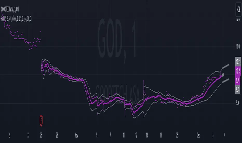
Elite By Ashu4750Inside Bar Detection:
The script identifies inside bars, which are candles where the high is lower and the low is higher than the previous bar. It tracks the high and low of the mother candle (the candle preceding the inside bars) and plots the ranges on the chart using lines and labels.
Exponential Moving Averages (EMA):
Three EMAs are calculated and plotted (with default periods of 9, 21, and 50). This is a classic trend-following technique used to smooth price data and identify the direction of the market.
Bollinger Bands (BB):
The script includes a Bollinger Band calculation using the simple moving average (SMA) with a standard deviation multiplier. The bands help visualize volatility and potential overbought or oversold conditions.
The user can configure settings like the length of the SMA and the multiplier for the upper and lower bands.
Volume Weighted Average Price (VWAP):
The VWAP is plotted on the chart and reset based on user-defined timeframes (e.g., session, week, month). VWAP is a popular indicator for institutional trading, as it shows the average price weighted by volume and can act as support or resistance.
Crossover Signals (Buy/Sell):
A combination of crossovers between VWAP, EMAs, and Bollinger Bands triggers buy and sell signals. Specifically:
Buy signal is generated when VWAP crosses over the 9 EMA, the close crosses over the Bollinger Band line, and VWAP crosses over the Bollinger Band.
Sell signal is triggered when VWAP crosses under the 9 EMA, and similar conditions exist for the other indicators.
These signals are plotted with a green "Buy" or red "Sell" marker below the bars, and alerts are set up for both buying and selling.
Additional Bollinger Band Configuration:
The script provides more flexibility in Bollinger Bands by allowing the user to select between SMA, EMA, or SMMA for the moving average.
The user can also choose the standard deviation multiplier and whether to display the bands.
Alerts:
Buy and sell conditions are linked to alert conditions, allowing the user to be notified when a signal is triggered, based on the defined crossover logic.
Technical Breakdown:
Inside Bar Logic: Tracks inside bars and plots lines representing the high and low of the mother candle. The line and label functions are used to draw these on the chart, which provides a visual representation of the range.
EMA and VWAP Crossovers:
The 9, 21, and 50-period EMAs are calculated and used in crossover logic with VWAP. Crossovers between VWAP and EMAs are a common method for identifying potential trend changes.
Bollinger Bands:
The Bollinger Band component allows for volatility analysis by calculating the upper and lower bands based on the moving average's standard deviation.
Alert System:
Alerts are set for crossover signals, allowing for real-time notifications of potential buy and sell opportunities.
Visualization:
The script plots the EMAs, VWAP, and Bollinger Bands on the price chart. It highlights inside bar patterns and displays buy/sell markers on the chart when the specified conditions are met. These visual cues make it easier to follow the market’s movements and spot trading opportunities.
Customizability:
The script is highly customizable with inputs for:
EMA periods.
VWAP settings.
Bollinger Band parameters (moving average type, length, standard deviation).
Candle color options for inside bars.
In this traders looking for multiple indicators to analyze market trends, volatility, and price action.

MCDX+RSI+SMA[THANHCONG]### Detailed Analysis of the MCDX+RSI+SMA Indicator
The MCDX+RSI+SMA indicator is designed to help investors conduct a deeper analysis of market trends by combining multiple technical factors into a single chart. This integration of popular indicators such as RSI, SMA, and Stochastic RSI provides investors with a comprehensive view of market movements, particularly in distinguishing between "Banker" and "Hot Money"—representing large and small capital flows.
#### Key Components of the Indicator:
1. **RSI for Banker and Hot Money:**
- **RSI (Relative Strength Index)** is a momentum oscillator that measures the speed and change of price movements, indicating overbought or oversold conditions. In this indicator, there are two distinct RSI lines configured for Banker (large capital) and Hot Money (small capital).
- Investors can adjust parameters like the RSI calculation period, baseline levels, and sensitivity for each type of capital flow, providing flexibility to adapt to varying market conditions.
2. **Moving Average (MA) of RSI:**
- The indicator employs two common types of Moving Averages: **SMA (Simple Moving Average)** and **EMA (Exponential Moving Average)**. These help smooth the RSI signals for Banker, offering a clearer view of the long-term trend of large capital in the market.
- Investors can select the type and period of the MA, allowing them to optimize the indicator for their trading style.
3. **Stochastic RSI:**
- The **Stochastic RSI** is incorporated to monitor overbought and oversold conditions over a specified timeframe. Parameters related to %K and %D of the Stochastic can also be adjusted to refine the accuracy of market signal analysis.
- A notable feature is the normalization of %K and %D on a 0-20 scale, making these lines compatible with other RSI charts, thus providing consistency in evaluating market strength.
4. **Overbought and Oversold Levels:**
- The indicator includes reference lines for overbought and oversold levels, aiding investors in identifying potential reversal zones in the market. This helps to avoid buying at excessively high prices or selling at excessively low prices.
#### Benefits for Investors:
- **Comprehensive View:** The indicator combines insights from both large (Banker) and small (Hot Money) capital flows, enabling investors to analyze not just trends but also the participation of each type of capital in the market.
- **Enhanced Technical Analysis:** By integrating multiple technical indicators within a single chart, investors can track important factors such as market momentum, overbought/oversold conditions, and capital flow shifts without needing to switch between various charts.
- **Flexibility and Customization:** The indicator allows adjustment of key parameters like the RSI period, sensitivity, type of MA, and Stochastic RSI settings, enabling investors to tailor the indicator to their trading strategy and timeframe.
- **Higher Reliability:** The combination of indicators like RSI, Stochastic RSI, and MA helps investors confirm trading signals more confidently. For instance, when both RSI and Stochastic RSI indicate overbought conditions, the likelihood of a reversal may be higher, reducing risk for investors.
#### Unique Features of the Indicator:
The MCDX+RSI+SMA indicator is a unique tool that integrates various market analysis factors into a single framework. This not only provides investors with a complete view of capital flows but also aids in optimizing decision-making based on multiple market aspects. Furthermore, its customizable parameters make it suitable for various trading strategies, from short-term to long-term.
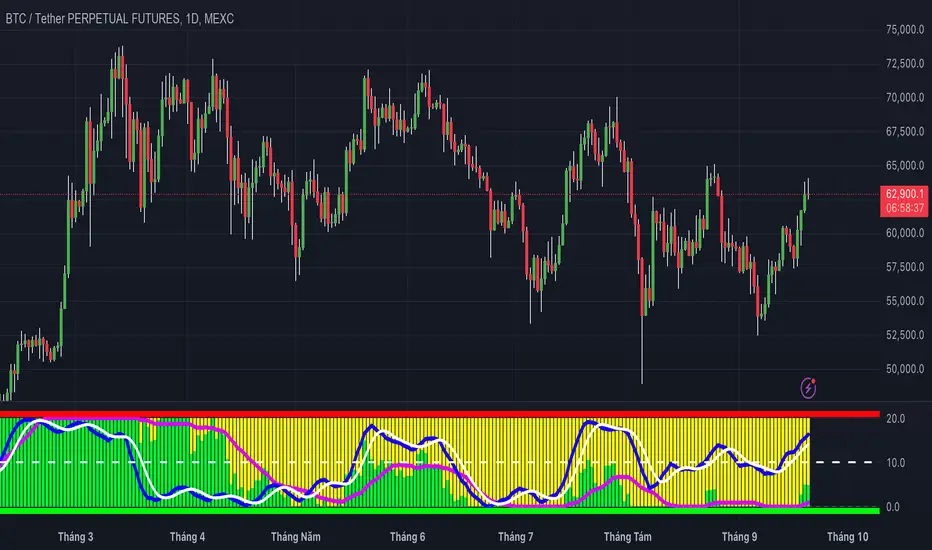
Multi-Sector Trend AnalysisThis script, titled "Multi-Sector Trend Analysis: Track Sector Momentum and Trends," is designed to assist traders and investors in monitoring multiple sectors of the stock market simultaneously. It leverages technical analysis by incorporating trend detection and momentum indicators like moving averages and the Relative Strength Index (RSI) to offer insights into the price action of various market sectors.
Core Features:
1. Sector-Based Analysis: The script covers 20 major sectors from the NSE (National Stock Exchange) such as Auto, Banking, Energy, FMCG, IT, Pharma, and others. Users can customize which sectors they wish to analyze using the available input fields.
Technical Indicators: The script uses two core technical indicators to detect trends and momentum:
2. Moving Averages: The script calculates both fast and slow exponential moving averages (EMAs). These are critical for identifying short- and long-term price trends and crossovers, helping detect shifts in momentum.
3. Relative Strength Index (RSI): A well-known momentum indicator that shows whether a stock is overbought or oversold. This script uses a 14-period RSI to gauge the strength of each sector.
4. Trend Detection: The script identifies whether the current market trend is "Up" or "Down" based on the relationship between the fast and slow EMAs (i.e., whether the fast EMA is above or below the slow EMA). It highlights this trend visually in a table format, allowing quick and easy trend recognition.
5. Gain/Loss Tracking: This feature calculates the percentage gain or loss since the last EMA crossover (a key point in trend change), giving users a sense of how much the price has moved since the trend shifted.
6. Customizable Table for Display: The script displays the analyzed data in a table format, where users can view each sector's:
Symbol
Trend (Up or Down)
RSI Value
Gain/Loss Since the Last EMA Crossover
This table is customizable in terms of size and color theme (dark or light), providing flexibility in presentation for different charting styles.
How It Works:
Sector Selection: Users can input up to 20 different sector symbols for analysis.
Moving Averages: Users can define the period lengths for both the fast and slow EMAs to suit their trading strategies.
Table Options: Choose between different table sizes and opt for a dark theme to enhance the visual appearance on charts.
How to Use:
Select the symbols (sectors) that you want to track. The script includes pre-configured symbols for major sectors on the NSE, but you can modify these to suit your needs.
Adjust the fast and slow EMA lengths to your preference. A common setting would be 3 for the fast EMA and 4 for the slow EMA, but more conservative traders might opt for higher values.
Customize the table size and theme based on your preference, whether you want a compact table or a larger one for easier readability.
Why Use This Script:
This script is ideal for traders looking to:
Monitor multiple market sectors simultaneously.
Identify key trends across sectors quickly.
Understand momentum and detect potential reversals through RSI and EMA crossovers.
Stay informed on sector performance using a clear visual table that tracks gains or losses.
By using this script, traders can gain better insights into sector-based trading strategies, improve their sector rotation tactics, and stay informed about the broader market environment. It provides a powerful yet easy-to-use tool for both beginner and advanced traders.

Uptrick: Dual Moving Average Volume Oscillator
Title: Uptrick: Dual Moving Average Volume Oscillator (DPVO)
### Overview
The "Uptrick: Dual Moving Average Volume Oscillator" (DPVO) is an advanced trading tool designed to enhance market analysis by integrating volume data with price action. This indicator is specially developed to provide traders with deeper insights into market dynamics, making it easier to spot potential entry and exit points based on volume and price interactions. The DPVO stands out by offering a sophisticated approach to traditional volume analysis, setting it apart from typical volume indicators available on the TradingView platform.
### Unique Features
Unlike traditional indicators that analyze volume and price movements separately, the DPVO combines these two critical elements to offer a comprehensive view of market behavior. By calculating the Volume Impact, which involves the product of the exponential moving averages (EMAs) of volume and the price range (close - open), this indicator highlights significant trading activities that could indicate strong buying or selling pressure. This method allows traders to see not just the volume spikes, but how those spikes relate to price movements, providing a clearer picture of market sentiment.
### Customization and Inputs
The DPVO is highly customizable, catering to various trading styles and strategies:
- **Oscillator Length (`oscLength`)**: Adjusts the period over which the volume and price difference is analyzed, allowing traders to set it according to their trading timeframe.
- **Fast and Slow Moving Averages (`fastMA` and `slowMA`)**: These parameters control the responsiveness of the DPVO. A shorter `fastMA` coupled with a longer `slowMA` can help in identifying trends quicker or smoothing out market noise for more conservative approaches.
- **Signal Smoothing (`signalSmooth`)**: This input helps in reducing signal noise, making the crossover and crossunder points between the DVO and its smoothed signal line clearer and easier to interpret.
### Functionality Details
The DPVO operates through a sequence of calculated steps that integrate volume data with price movement:
1. **Volume Impact Calculation**: This is the foundational step where the product of the EMA of volume and the EMA of price range (close - open) is calculated. This metric highlights trading sessions where significant volume accompanies substantial price movements, suggesting a strong market response.
2. **Dynamic Volume Oscillator (DVO)**: The heart of the indicator, the DVO, is derived by calculating the difference between the fast EMA and the slow EMA of the Volume Impact. This result is then normalized by dividing by the EMA of the volume over the same period to scale the output, making it consistent across various trading environments.
3. **Signal Generation**: The final output is smoothed using a simple moving average of the DVO to filter out market noise. Buy and sell signals are generated based on the crossover and crossunder of the DVO with its smoothed version, providing clear cues for market entry or exit.
### Originality
The DPVO's originality lies in its innovative integration of volume and price movement, a novel approach not typically observed in other volume indicators. By analyzing the product of volume and price change EMAs, the DPVO captures the essence of market dynamics more holistically than traditional tools, which often only reflect volume levels without contextualizing them with price actions. This dual analysis provides traders with a deeper understanding of market forces, enabling them to make more informed decisions based on a combination of volume surges and significant price movements. The DPVO also introduces a unique normalization and smoothing technique that refines the oscillator's output, offering cleaner and more reliable signals that are adaptable to various market conditions and trading styles.
### Practical Application
The DPVO excels in environments where volume plays a crucial role in validating price movements. Traders can utilize the buy and sell signals generated by the DPVO to enhance their decision-making process. The signals are plotted directly on the trading chart, with buy signals appearing below the price bars and sell signals above, ensuring they are prominent and actionable. This setup is particularly useful for day traders and swing traders who rely on timely and accurate signals to maximize their trading opportunities.
### Best Practices
To maximize the effectiveness of the DPVO, traders should consider the following best practices:
- **Market Selection**: Use the DPVO in markets known for strong volume-price correlation such as major forex pairs, popular stocks, and cryptocurrencies.
- **Signal Confirmation**: While the DPVO provides powerful signals, confirming these signals with additional indicators such as RSI or MACD can increase trade reliability.
- **Risk Management**: Always use stop-loss orders to manage risks associated with trading signals. Adjust the position size based on the volatility of the asset to avoid significant losses.
### Practical Example + How to use it
Practical Example1: Day Trading Cryptocurrencies
For a day trader focusing on the highly volatile cryptocurrency market, the DPVO can be an effective tool on a 15-minute chart. Suppose a trader is monitoring Bitcoin (BTC) during a period of high market activity. The DPVO might show an upward crossover of the DVO above its smoothed signal line while also indicating a significant increase in volume. This could signal that strong buying pressure is entering the market, suggesting a potential short-term rally. The trader could enter a long position based on this signal, setting a stop-loss just below the recent support level to manage risk. If the DPVO later shows a crossover in the opposite direction with decreasing volume, it might signal a good exit point, allowing the trader to lock in profits before a potential pullback.
- **Swing Trading Stocks**: For a swing trader looking at stocks, the DPVO could be applied on a daily chart. If the oscillator shows a consistent downward trend along with increasing volume, this could suggest a potential sell-off, providing a sell signal before a significant downturn.
You can look for:
--> Increase in volume - You can use indicators like 24-hour-Volume to have a better visualization
--> Uptrend/Downtrend in the indicator (HH, HL, LL, LH)
--> Confirmation (Buy signal/Sell signal)
--> Correct Price action (Not too steep moves up or down. Stable moves.) (Optional)
--> Confirmation with other indicators (Optional)
Quick image showing you an example of a buy signal on SOLANA:
### Technical Notes
- **Calculation Efficiency**: The DPVO utilizes exponential moving averages (EMAs) in its calculations, which provides a balance between responsiveness and smoothing. EMAs are favored over simple moving averages in this context because they give more weight to recent data, making the indicator more sensitive to recent market changes.
- **Normalization**: The normalization of the DVO by the EMA of the volume ensures that the oscillator remains consistent across different assets and timeframes. This means the indicator can be used on a wide variety of markets without needing significant adjustments, making it a versatile tool for traders.
- **Signal Line Smoothing**: The final signal line is smoothed using a simple moving average (SMA) to reduce noise. The choice of SMA for smoothing, as opposed to EMA, is intentional to provide a more stable signal that is less prone to frequent whipsaws, which can occur in highly volatile markets.
- **Lag and Sensitivity**: Like all moving average-based indicators, the DPVO may introduce a slight lag in signal generation. However, this is offset by the indicator’s ability to filter out market noise, making it a reliable tool for identifying genuine trends and reversals. Adjusting the `fastMA`, `slowMA`, and `signalSmooth` inputs allows traders to fine-tune the sensitivity of the DPVO to match their specific trading strategy and market conditions.
- **Platform Compatibility**: The DPVO is written in Pine Script™ v5, ensuring compatibility with the latest features and functionalities offered by TradingView. This version takes advantage of optimized functions for performance and accuracy in calculations, making it well-suited for real-time analysis.
Conclusion
The "Uptrick: Dual Moving Average Volume Oscillator" is a revolutionary tool that merges volume analysis with price movement to offer traders a more nuanced understanding of market trends and reversals. Its ability to provide clear, actionable signals based on a unique combination of volume and price changes makes it an invaluable addition to any trader's toolkit. Whether you are managing long-term positions or looking for quick trades, the DPVO provides insights that can help refine any trading strategy, making it a standout choice in the crowded field of technical indicators.
Nothing from this indicator or any other Uptrick Indicators is financial advice. Only you are ultimately responsible for your choices.
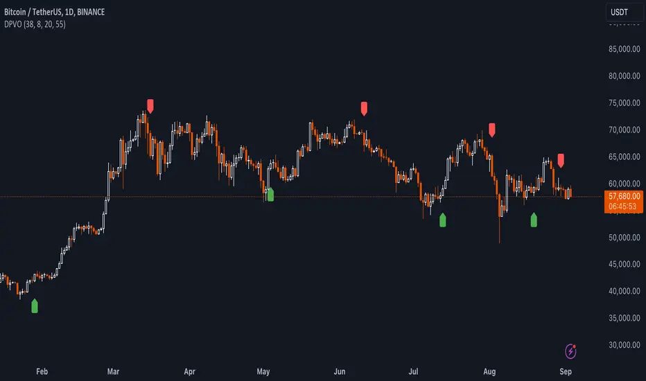
Support and resistance levels (Day, Week, Month) + EMAs + SMAs(ENG): This Pine 5 script provides various tools for configuring and displaying different support and resistance levels, as well as moving averages (EMA and SMA) on charts. Using these tools is an essential strategy for determining entry and exit points in trades.
Support and Resistance Levels
Daily, weekly, and monthly support and resistance levels play a key role in analyzing price movements:
Daily levels: Represent prices where a cryptocurrency has tended to bounce within the current trading day.
Weekly levels: Reflect strong prices that hold throughout the week.
Monthly levels: Indicate the most significant levels that can influence price movement over the month.
When trading cryptocurrencies, traders use these levels to make decisions about entering or exiting positions. For example, if a cryptocurrency approaches a weekly resistance level and fails to break through it, this may signal a sell opportunity. If the price reaches a daily support level and starts to bounce up, it may indicate a potential long position.
Market context and trading volumes are also important when analyzing support and resistance levels. High volume near a level can confirm its significance and the likelihood of subsequent price movement. Traders often combine analysis across different time frames to get a more complete picture and improve the accuracy of their trading decisions.
Moving Averages
Moving averages (EMA and SMA) are another important tool in the technical analysis of cryptocurrencies:
EMA (Exponential Moving Average): Gives more weight to recent prices, allowing it to respond more quickly to price changes.
SMA (Simple Moving Average): Equally considers all prices over a given period.
Key types of moving averages used by traders:
EMA 50 and 200: Often used to identify trends. The crossing of the 50-day EMA with the 200-day EMA is called a "golden cross" (buy signal) or a "death cross" (sell signal).
SMA 50, 100, 150, and 200: These periods are often used to determine long-term trends and support/resistance levels. Similar to the EMA, the crossings of these averages can signal potential trend changes.
Settings Groups:
EMA Golden Cross & Death Cross: A setting to display the "golden cross" and "death cross" for the EMA.
EMA 50 & 200: A setting to display the 50-day and 200-day EMA.
Support and Resistance Levels: Includes settings for daily, weekly, and monthly levels.
SMA 50, 100, 150, 200: A setting to display the 50, 100, 150, and 200-day SMA.
SMA Golden Cross & Death Cross: A setting to display the "golden cross" and "death cross" for the SMA.
Components:
Enable/disable the display of support and resistance levels.
Show level labels.
Parameters for adjusting offset, display of EMA and SMA, and their time intervals.
Parameters for configuring EMA and SMA Golden Cross & Death Cross.
EMA Parameters:
Enable/disable the display of 50 and 200-day EMA.
Color and style settings for EMA.
Options to use bar gaps and the "LookAhead" function.
SMA Parameters:
Enable/disable the display of 50, 100, 150, and 200-day SMA.
Color and style settings for SMA.
Options to use bar gaps and the "LookAhead" function.
Effective use of support and resistance levels, as well as moving averages, requires an understanding of technical analysis, discipline, and the ability to adapt the strategy according to changing market conditions.
(RUS) Данный Pine 5 скрипт предоставляет разнообразные инструменты для настройки и отображения различных уровней поддержки и сопротивления, а также скользящих средних (EMA и SMA) на графиках. Использование этих инструментов является важной стратегией для определения точек входа и выхода из сделок.
Уровни поддержки и сопротивления
Дневные, недельные и месячные уровни поддержки и сопротивления играют ключевую роль в анализе движения цен:
Дневные уровни: Представляют собой цены, на которых криптовалюта имела тенденцию отскакивать в течение текущего торгового дня.
Недельные уровни: Отражают сильные цены, которые сохраняются в течение недели.
Месячные уровни: Указывают на наиболее значимые уровни, которые могут влиять на движение цены в течение месяца.
При торговле криптовалютами трейдеры используют эти уровни для принятия решений о входе в позицию или закрытии сделки. Например, если криптовалюта приближается к недельному уровню сопротивления и не удается его преодолеть, это может стать сигналом для продажи. Если цена достигает дневного уровня поддержки и начинает отскакивать вверх, это может указывать на возможность открытия длинной позиции.
Контекст рынка и объемы торговли также важны при анализе уровней поддержки и сопротивления. Высокий объем при приближении к уровню может подтвердить его значимость и вероятность последующего движения цены. Трейдеры часто комбинируют анализ различных временных рамок для получения более полной картины и улучшения точности своих торговых решений.
Скользящие средние
Скользящие средние (EMA и SMA) являются еще одним важным инструментом в техническом анализе криптовалют:
EMA (Exponential Moving Average): Экспоненциальная скользящая средняя, которая придает большее значение последним ценам. Это позволяет более быстро реагировать на изменения в ценах.
SMA (Simple Moving Average): Простая скользящая средняя, которая равномерно учитывает все цены в заданном периоде.
Основные виды скользящих средних, которые используются трейдерами:
EMA 50 и 200: Часто используются для выявления трендов. Пересечение 50-дневной EMA с 200-дневной EMA называется "золотым крестом" (сигнал на покупку) или "крестом смерти" (сигнал на продажу).
SMA 50, 100, 150 и 200: Эти периоды часто используются для определения долгосрочных трендов и уровней поддержки/сопротивления. Аналогично EMA, пересечения этих средних могут сигнализировать о возможных изменениях тренда.
Группы настроек:
EMA Golden Cross & Death Cross: Настройка для отображения "золотого креста" и "креста смерти" для EMA.
EMA 50 & 200: Настройка для отображения 50-дневной и 200-дневной EMA.
Уровни поддержки и сопротивления: Включает настройки для дневных, недельных и месячных уровней.
SMA 50, 100, 150, 200: Настройка для отображения 50, 100, 150 и 200-дневных SMA.
SMA Golden Cross & Death Cross: Настройка для отображения "золотого креста" и "креста смерти" для SMA.
Компоненты:
Включение/отключение отображения уровней поддержки и сопротивления.
Показ ярлыков уровней.
Параметры для настройки смещения, отображения EMA и SMA, а также их временных интервалов.
Параметры для настройки EMA и SMA Golden Cross & Death Cross.
Параметры EMA:
Включение/отключение отображения 50 и 200-дневных EMA.
Настройки цвета и стиля для EMA.
Опции для использования разрыва баров и функции "LookAhead".
Параметры SMA:
Включение/отключение отображения 50, 100, 150 и 200-дневных SMA.
Настройки цвета и стиля для SMA.
Опции для использования разрыва баров и функции "LookAhead".
Эффективное использование уровней поддержки и сопротивления, а также скользящих средних, требует понимания технического анализа, дисциплины и умения адаптировать стратегию в зависимости от изменяющихся условий рынка.

Strong Support and Resistance with EMAs @viniciushadek
### Strategy for Using Continuity Points with 20 and 9 Period Exponential Moving Averages, and Support and Resistance
This strategy involves using two exponential moving averages (EMA) - one with a 20-period and another with a 9-period - along with identifying support and resistance levels on the chart. Combining these tools can help determine trend continuation points and potential entry and exit points in market operations.
### 1. Setting Up the Exponential Moving Averages
- **20-Period EMA**: This moving average provides a medium-term trend view. It helps smooth out price fluctuations and identify the overall market direction.
- **9-Period EMA**: This moving average is more sensitive and reacts more quickly to price changes, providing short-term signals.
### 2. Identifying Support and Resistance
- **Support**: Price levels where demand is strong enough to prevent the price from falling further. These levels are identified based on previous lows.
- **Resistance**: Price levels where supply is strong enough to prevent the price from rising further. These levels are identified based on previous highs.
### 3. Continuity Points
The strategy focuses on identifying trend continuation points using the interaction between the EMAs and the support and resistance levels.
### 4. Buy Signals
- When the 9-period EMA crosses above the 20-period EMA.
- Confirm the entry if the price is near a support level or breaking through a resistance level.
### 5. Sell Signals
- When the 9-period EMA crosses below the 20-period EMA.
- Confirm the exit if the price is near a resistance level or breaking through a support level.
### 6. Risk Management
- Use appropriate stops below identified supports for buy operations.
- Use appropriate stops above identified resistances for sell operations.
### 7. Validating the Trend
- Check if the trend is validated by other technical indicators, such as the Relative Strength Index (RSI) or Volume.
### Conclusion
This strategy uses the combination of exponential moving averages and support and resistance levels to identify continuity points in the market trend. It is crucial to confirm the signals with other technical analysis tools and maintain proper risk management to maximize results and minimize losses.
Implementing this approach can provide a clearer view of market movements and help make more informed trading decisions.
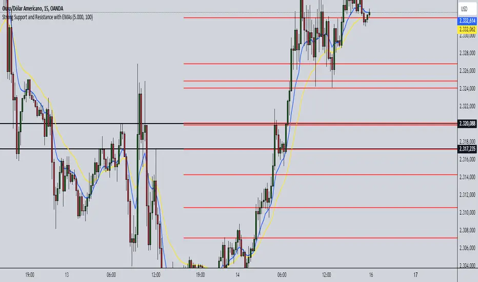
Moving Average Bands with Signals [UAlgo]The "Moving Average Bands with Signals combines various moving average types with ATR-based bands to help traders identify potential support and resistance levels.
It plots moving average bands with upper and lower support/resistance levels based on the Average True Range (ATR) and user-defined settings.Additionally, the script generates buy/sell signals based on price crossing above or below the bands.
🔶 Key Features
Multiple Moving Average Types:
Supports various moving average calculations including Arnaud Legoux Moving Average (ALMA), Exponential Moving Average (EMA), Double Exponential Moving Average (DEMA), Triple Exponential Moving Average (TEMA), Kaufman Adaptive Moving Average (KAMA), Hull Moving Average (HMA), Least Squares Moving Average (LSMA), Simple Moving Average (SMA), Triangular Moving Average (TMA), Volume-Weighted Moving Average (VWMA), Weighted Moving Average (WMA), and Zero-Lag Moving Average (ZLMA).
Customizable ATR Bands:
Integrates the Average True Range (ATR) to calculate dynamic support and resistance bands around the moving average. The multiplier for the bands is user-adjustable, allowing for finer control over the sensitivity and width of the bands.
Signal Generation:
Provides visual signals on the chart when the price interacts with the support or resistance bands. Users can choose between using the wick or the close price to generate these signals, adding an extra layer of customization based on their trading style.
Flexible Input Parameters:
Allows users to input parameters for moving average length, ATR length, band multiplier, and signal type. Additional settings are available for specific moving average types, such as ALMA's offset and sigma, KAMA's fast and slow periods, and LSMA's offset.
🔶 Disclaimer
This script is provided for educational purposes only and should not be considered financial advice.
Trading financial instruments involves substantial risk and can result in significant financial losses.
The script’s performance in the past is not indicative of future results, and no guarantees are made regarding its accuracy, reliability, or performance.

Support Resistance & Ema
The "Support Resistance & Ema" indicator combines various strategies to assist traders in identifying significant support and resistance levels on the chart and in following trends through exponential moving averages (EMA). This script is designed to be versatile and useful in different trading strategies.
Key Features:
Support and Resistance: It utilizes pivot highs and lows to pinpoint support and resistance levels. These levels are plotted on the chart with lines that change color based on trend reversals.
Trend Identification: The indicator follows trends using four conditions:
_hh: Higher highs and higher lows, indicating an uptrend.
_ll: Lower highs and lower lows, indicating a downtrend.
_hl: Higher highs and lower lows, indicating weakening uptrend or an impending reversal.
_lh: Lower highs and higher lows, indicating weakening downtrend or an impending reversal.
Exponential Moving Averages (EMA): It also displays various EMAs (9, 21, 50, 100, 200) on the chart to provide further insights into the trend direction.
Usage:
Support and Resistance: Support and resistance lines are automatically plotted on the chart. Trend reversals are highlighted by changing the color of the lines.
Trend Identification: The _hh, _ll, _hl, _lh conditions help identify trend changes. When one of these conditions is met, it indicates a particular configuration of highs and lows that might suggest a trading opportunity.
Exponential Moving Averages (EMA): The EMAs are plotted on the chart and can be used to confirm trends identified by the main indicator.
To use this script, you need to add it as an indicator to your trading chart. Once applied, the support, resistance lines, and EMAs will be visible on the chart, providing traders with valuable information to make informed trading decisions.
In summary, this script offers a comprehensive way to identify significant support and resistance levels, spot market trends, and confirm those trends through the use of exponential moving averages.
